AE 14: Modeling Housing Prices 🏠

In this application exercise we will be studying housing prices. The dataset is a cleaned version of publicly available real estate data. We will use tidyverse and tidymodels for data exploration and modeling, respectively.

library(tidyverse)
library(tidymodels)
library(modeldata)

We will use the ames_housing dataset from the modeldata package.

Before we use the dataset, we’ll make a few transformations to it.

Your turn: Review the code below with your neighbors and write a summary of the data transformation pipeline.

data(ames)
housing <- ames |>
  select(Sale_Price, Gr_Liv_Area, Bldg_Type, Bedroom_AbvGr, Paved_Drive, Exter_Cond) |>
  mutate(home_type = fct_collapse(Bldg_Type,
    "House" = c("OneFam", "TwnhsE"),
    "Townhouse" = "Twnhs",
    "Duplex" = "Duplex"
  )) |>
  select(-Bldg_Type) |>
  rename(price = Sale_Price, sqft = Gr_Liv_Area, bedrooms = Bedroom_AbvGr) |>
  filter(home_type %in% c("House", "Townhouse", "Duplex"))

Here is a glimpse at the data:

glimpse(housing)

Rows: 2,868
Columns: 6
$ price       <int> 215000, 105000, 172000, 244000, 189900, 195500, 213500, 19…
$ sqft        <int> 1656, 896, 1329, 2110, 1629, 1604, 1338, 1280, 1616, 1804,…
$ bedrooms    <int> 3, 2, 3, 3, 3, 3, 2, 2, 2, 3, 3, 3, 3, 2, 1, 4, 4, 1, 2, 3…
$ Paved_Drive <fct> Partial_Pavement, Paved, Paved, Paved, Paved, Paved, Paved…
$ Exter_Cond  <fct> Typical, Typical, Typical, Typical, Typical, Typical, Typi…
$ home_type   <fct> House, House, House, House, House, House, House, House, Ho…

Get to know the data

Your turn: What is a typical house price in this dataset? What are some common square footage values? What types of homes are most common? Additionally, explore at least 1-2 other features that could be interesting. Share your findings!

# add code here

Price vs. square footage

How can we use square footage to model/predict pricing? Here is the model:

price_sqft_fit <- linear_reg() |>
  fit(price ~ sqft, data = housing)

tidy(price_sqft_fit)

# A tibble: 2 × 5
  term        estimate std.error statistic  p.value
  <chr>          <dbl>     <dbl>     <dbl>    <dbl>
1 (Intercept)   11430.   3271.        3.49 0.000482
2 sqft            114.      2.07     55.0  0

And here is the model visualized:

ggplot(housing, aes(x = sqft, y = price)) +
  geom_point(alpha = 0.4) +
  geom_smooth(method = "lm")

`geom_smooth()` using formula = 'y ~ x'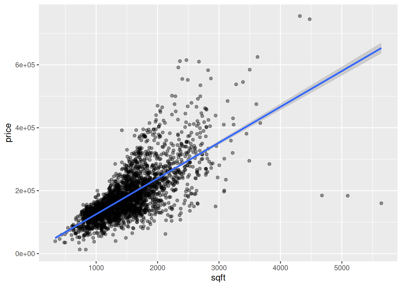

Your turn: Write the fitted equation of the model in mathematical notation. Then, interpret the intercept and slope.

\[ add~equation~here \]

Price vs. home type

price_type_fit <- linear_reg() |>
  fit(price ~ home_type, data = housing)

tidy(price_type_fit)

# A tibble: 3 × 5
  term               estimate std.error statistic  p.value
  <chr>                 <dbl>     <dbl>     <dbl>    <dbl>
1 (Intercept)         185469.     1537.    121.   0       
2 home_typeDuplex     -45661.     7746.     -5.89 4.20e- 9
3 home_typeTownhouse  -49535.     8036.     -6.16 8.06e-10

Your turn: Write the fitted equation of the model in mathematical notation. Then, interpret the intercept and each coefficient in context.

\[ add~equation~here \]

Price vs. square footage and home type

Now, let’s fit a model that use both variables!

Main effects model

The main effects model is another name for the additive model. Here is the model:

price_main_fit <- linear_reg() |>
  fit(price ~ sqft + home_type, data = housing)

tidy(price_main_fit)

# A tibble: 4 × 5
  term               estimate std.error statistic  p.value
  <chr>                 <dbl>     <dbl>     <dbl>    <dbl>
1 (Intercept)          13395.   3225.        4.15 3.38e- 5
2 sqft                   115.      2.03     56.5  0       
3 home_typeDuplex     -63251.   5338.      -11.8  1.19e-31
4 home_typeTownhouse  -20306.   5552.       -3.66 2.60e- 4

Your turn: Write the fitted equation of the model in mathematical notation. Then, interpret the intercept and each slope coefficient.

\[ add~equation~here \]

Interaction effects model

Now, we will fit an interaction effects model.

Task: Write code to fit an interaction effects model predicting price from square footage and home type.

#add code here

Task: Write the fitted equation using mathematical notation.

\[ add~equation~here \]

Task: Write the fitted equations for each home type.

\[ add~equation~here \] \[ add~equation~here \] \[ add~equation~here \]

Model Comparison

So, we fit multiple models - how do we know which one is better?

Using glance(), report each of the above models’ adjusted \(R^2\) values.

Which model is the best fit? Which is the worst?

# add code here

One more model?

Task: Try adding one more variable present in the data frame to the “best” model chosen above. Does it make a difference in adjusted \(R^2\)? What about plain old \(R^2\)?

# add code here