# A tibble: 8 × 4
# Groups:   flip18 [3]
  flip18 gerry     n  prop
   <dbl> <fct> <int> <dbl>
1     -1 low       2 0.4
2     -1 mid       3 0.6
3      0 low      52 0.133
4      0 mid     242 0.617
5      0 high     98 0.25
6      1 low       8 0.211
7      1 mid      25 0.658
8 1 high 5 0.132Exploratory Data Analysis II
Lecture 5
Katie Solarz
Duke University
STA 199 Summer 2026: Session I
May 10, 2026
Announcements/Reminders
Lab is due TONIGHT at 11:59PM ➞ submit PDF to Gradescope
Come to office hours and/or post on Ed for help!
Kenna’s office hours are 11:00am - 1:00pm today on Zoom (find link on Canvas)
Always double check your project (top right-hand corner of screen in your RStudio) & be sure you are in the correct project for the task at hand (AE in lecture, lab in lab / at home when working on assignments)
Exam Intel
Midterm Date: Monday, 6/1 (confirmed)
Exam will take place during both lecture & lab time slots (i.e., you will have from 9:30am - 12:15pm)
I am NOT writing an exam I expect to take the full 2hr 45min timeframe; having the exam during both lecture & lab is meant to take some of the time pressure away from the exam & allow buffer time in case of any technical issues
You are of course entitled to the full 2hr 45min if you need it!
Format: written portion (mult. choice) & live coding / free response (think about this as a short lab assignment) on your laptop
Once you are finished with the written portion, you will turn it in and clone an exam repo
Cheatsheet (standard printer paper, both sides, can be hand-written/typed/combo, idc) allowed for both portions of the exam
The coding portion of the exam is open-assignment in that you will be working in your containers, so you have access to all of your AEs & lab assignments by changing projects (of course, switching between projects and looking through these materials eats away at time, so I wouldn’t be entirely reliant on this)
The coding portion of the exam will be closed-internet (i.e., you cannot open any other tabs on your browser aside from GitHub & your container); myself, Kenna, and potentially one additional person will be proctoring and actively monitoring adherence to this policy (breaking this policy will result in a score of 0 for this portion of the exam)
I will provide review materials for both portions ahead of time (likely by next Thursday) – your labs are the best preparatory materials, so make sure you feel confident with all lab content & review your graded feedback!
If you need accommodations and I have not received a letter, please get it to me by EOD today; make your appointment in the testing center!
Questions??
Lab: Narrative
-
Boxplots, histograms, density plots:
Center: Give an idea of a ‘typical value’ (median or mean, most commonly; choose which you think is more appropriate for the data, or mention both!);
Spread: Does the data have a lot of variability (“wide, flat” distribution), or just a little (“narrow” distribution)? What is the primary range of the data? (IQR, outliers)
Shape: Is there skew, or is the distribution symmetric? If the data are skewed, in which direction? Is the distribution unimodal, bimodal, or multimodal?
Outliers: Are there any unsual data points (whether via visual or mathematical assessment (i.e., “dots” on a boxplot))
Lab: Narrative
-
Scatter Plots
Is there a relationship between the two variables? Is it positive or negative?
If there is a relationship, does it seem to be strong or weak?
Is the relationship linear or nonlinear (i.e., quadratic, exponential, logarithmic)?
Lab: Advice
Be Specific in your narrative. Don’t just say “the spread is small and the center is low” What does that mean??? Give numbers, units (if available), etc.
Be Specific in your plot labels
Answer all parts of the question!! Statements like “Compare…” mean to do so in the written answer!
Written answers should be text outside of code chunks, not comments
Make sure you can render to PDF early & often :) This will help you identify / troubleshoot issues with your code that may not be apparent in isolation
Outline
Monday: Started learning about data transformation & intro to piping
Yesterday: More (gg)plotting & describing distributions
-
Today:
Review from last time + finish AE04
More about the pipe
Transformation + plotting combo
AE-04
Quick Review: Data Viz
After a while this is more art than science, but you can narrow down the options based on the number and type of variables:
| Variable combo | Options |
|---|---|
| 1 numerical | histogram, density, box plot |
| 1 categorical | bar chart, |
| 2 numerical | scatterplot |
| numerical/categorical | side-by-side box or violin plots, stacked densities or histograms |
| 2 categorical | stacked bar plot (today) |
For three or more variables, the human mind is limited, and you have to start getting creative (play with color, texture, etc).
Quick Review: Row operations
-
slice(): chooses rows based on location
-
filter(): chooses rows based on column values
-
arrange(): changes the order of the rows
-
sample_n(): take a random subset of the rows
| X1 | X2 | X3 |
|---|---|---|
| 1 | a | yes |
| 3 | b | no |
| 5 | a | yes |
| 7 | b | yes |
| 9 | a | yes |
Quick Review: Column operations
-
select(): changes whether or not a column is included
-
rename(): changes the name of columns
-
mutate(): changes the values of columns and creates new columns
| X1 | X2 | X3 |
|---|---|---|
| 1 | a | yes |
| 3 | b | no |
| 5 | a | yes |
| 7 | b | yes |
| 9 | a | yes |
Quick Review: Groups of rows
-
summarize(): collapses a group into a single row
-
count(): count unique values of one or more variables
-
group_by(): perform calculations separately for each value of a variable
| X1 | X2 | X3 |
|---|---|---|
| 1 | a | yes |
| 3 | b | no |
| 5 | a | yes |
| 7 | b | yes |
| 9 | a | yes |
Drilling down:
group_by(),
summarize(),
count()
What does group_by() do?
What does group_by() do in the following pipeline?
What does group_by() do?
What does group_by() do in the following pipeline?
Let’s simplify!
What does group_by() do in the following pipeline?
Let’s simplify!
What does group_by() do in the following pipeline?
group_by()
it converts a data frame to a grouped data frame, where subsequent operations are performed once per group
ungroup()removes grouping
# A tibble: 435 × 12
# Groups: state [50]
district last_name first_name party16 clinton16 trump16 dem16 state
<chr> <chr> <chr> <chr> <dbl> <dbl> <dbl> <chr>
1 AK-AL Young Don R 37.6 52.8 0 AK
2 AL-01 Byrne Bradley R 34.1 63.5 0 AL
3 AL-02 Roby Martha R 33 64.9 0 AL
4 AL-03 Rogers Mike D. R 32.3 65.3 0 AL
5 AL-04 Aderholt Rob R 17.4 80.4 0 AL
6 AL-05 Brooks Mo R 31.3 64.7 0 AL
7 AL-06 Palmer Gary R 26.1 70.8 0 AL
8 AL-07 Sewell Terri D 69.8 28.6 1 AL
9 AR-01 Crawford Rick R 30.2 65 0 AR
10 AR-02 Hill French R 41.7 52.4 0 AR
# ℹ 425 more rows
# ℹ 4 more variables: party18 <chr>, dem18 <dbl>, flip18 <dbl>,
# gerry <fct>group_by()
it converts a data frame to a grouped data frame, where subsequent operations are performed once per group
ungroup()removes grouping
# A tibble: 435 × 12
district last_name first_name party16 clinton16 trump16 dem16 state
<chr> <chr> <chr> <chr> <dbl> <dbl> <dbl> <chr>
1 AK-AL Young Don R 37.6 52.8 0 AK
2 AL-01 Byrne Bradley R 34.1 63.5 0 AL
3 AL-02 Roby Martha R 33 64.9 0 AL
4 AL-03 Rogers Mike D. R 32.3 65.3 0 AL
5 AL-04 Aderholt Rob R 17.4 80.4 0 AL
6 AL-05 Brooks Mo R 31.3 64.7 0 AL
7 AL-06 Palmer Gary R 26.1 70.8 0 AL
8 AL-07 Sewell Terri D 69.8 28.6 1 AL
9 AR-01 Crawford Rick R 30.2 65 0 AR
10 AR-02 Hill French R 41.7 52.4 0 AR
# ℹ 425 more rows
# ℹ 4 more variables: party18 <chr>, dem18 <dbl>, flip18 <dbl>,
# gerry <fct>group_by() |> summarize()
A common pipeline is group_by() and then summarize() to calculate summary statistics for each group:
gerrymander |>
group_by(state) |>
summarize(
mean_trump16 = mean(trump16),
median_trump16 = median(trump16)
)# A tibble: 50 × 3
state mean_trump16 median_trump16
<chr> <dbl> <dbl>
1 AK 52.8 52.8
2 AL 62.6 64.9
3 AR 60.9 63.0
4 AZ 46.9 47.7
5 CA 31.7 28.4
6 CO 43.6 41.3
7 CT 41.0 40.4
8 DE 41.9 41.9
9 FL 47.9 49.6
10 GA 51.3 56.6
# ℹ 40 more rowsgroup_by() |> summarize()
This pipeline can also be used to count number of observations for each group:
summarize()
summarize()
Recall from yesterday…
gerrymander |>
summarize(
mean_trump_perc = mean(trump16),
median_trump_perc = median(trump16),
sd = sd(trump16),
iqr = IQR(trump16),
q25 = quantile(trump16, 0.25),
q75 = quantile(trump16, 0.75)
)# A tibble: 1 × 6
mean_trump_perc median_trump_perc sd iqr q25 q75
<dbl> <dbl> <dbl> <dbl> <dbl> <dbl>
1 45.9 48.7 16.8 23.3 34.8 58.1summarize()
Or, more concisely
summarize()
Getting to the point…
-
summarize()creates a new data frame that stores the summaries; - You can compute as many summaries as you want, and whichever you want, in a single call to
summarize(); - To the left of the equal signs are your choice of column names in the new data frame you are creating. You can type whatever you want here (within reason);
- To the right of the equal signs is
Rcode that computes the summaries. You must use the correct command names (case sensitive):mean,median,quantile,sd,var, etc; - If you want to learn what these do, read the documentation (eg
?quantile).
Spot the difference
What’s the difference between the following two pipelines?
Spot the difference

count()
Count the number of observations in each level of variable(s); if you supply more than 1 variable, count the number of observations in each unique combination of levels across all variables
Place the counts in a variable called
n; you can access this variable in downstream code
count() and sort
What does the following pipeline do? Rewrite it with count() instead.
count() and sort
What does the following pipeline do? Rewrite it with count() instead.
count() and sort
What does the following pipeline do? Rewrite it with count() instead.
mutate()
Flip the question
Note
From AE-04: Is a Congressional District more likely to have high prevalence of gerrymandering if a Democrat was able to flip the seat in the 2018 election?
vs.
Note
Is a Congressional District more likely to be flipped to a Democratic seat if it has high prevalence of gerrymandering or low prevalence of gerrymandering?
Flipping vs. gerrymandering prevalence
The following code should produce a visualization that answers the question “Is a Congressional District more likely to be flipped to a Democratic seat if it has high prevalence of gerrymandering or low prevalence of gerrymandering?” However, it produces a warning and an unexpected plot. What’s going on?
Warning: The following aesthetics were dropped during statistical
transformation: fill.
ℹ This can happen when ggplot fails to infer the correct grouping
structure in the data.
ℹ Did you forget to specify a `group` aesthetic or to convert a
numerical variable into a factor?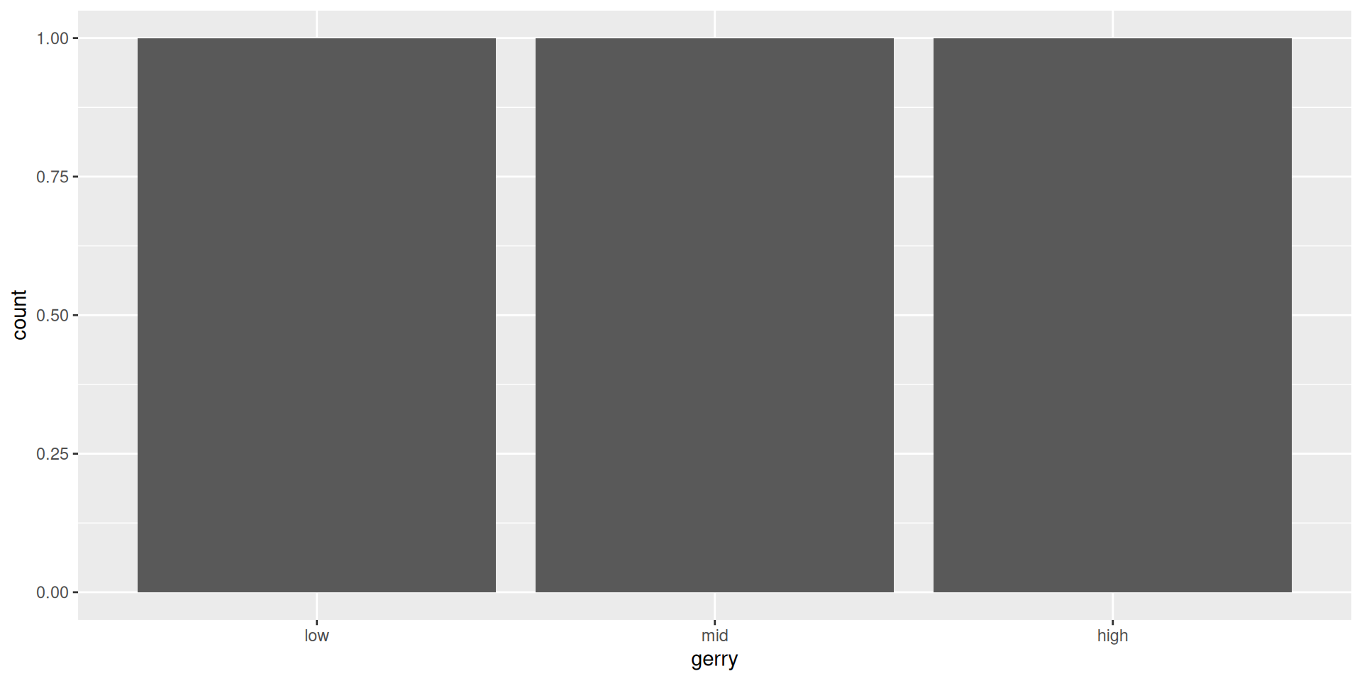
Another glimpse at gerrymander
Rows: 435
Columns: 12
$ district <chr> "AK-AL", "AL-01", "AL-02", "AL-03", "AL-04", "AL-…
$ last_name <chr> "Young", "Byrne", "Roby", "Rogers", "Aderholt", "…
$ first_name <chr> "Don", "Bradley", "Martha", "Mike D.", "Rob", "Mo…
$ party16 <chr> "R", "R", "R", "R", "R", "R", "R", "D", "R", "R",…
$ clinton16 <dbl> 37.6, 34.1, 33.0, 32.3, 17.4, 31.3, 26.1, 69.8, 3…
$ trump16 <dbl> 52.8, 63.5, 64.9, 65.3, 80.4, 64.7, 70.8, 28.6, 6…
$ dem16 <dbl> 0, 0, 0, 0, 0, 0, 0, 1, 0, 0, 0, 0, 1, 0, 1, 0, 0…
$ state <chr> "AK", "AL", "AL", "AL", "AL", "AL", "AL", "AL", "…
$ party18 <chr> "R", "R", "R", "R", "R", "R", "R", "D", "R", "R",…
$ dem18 <dbl> 0, 0, 0, 0, 0, 0, 0, 1, 0, 0, 0, 0, 1, 1, 1, 0, 0…
$ flip18 <dbl> 0, 0, 0, 0, 0, 0, 0, 0, 0, 0, 0, 0, 0, 1, 0, 0, 0…
$ gerry <fct> mid, high, high, high, high, high, high, high, mi…mutate()
We want to use
flip18as a categorical variableBut it’s stored as a numeric
So we need to change its type first, before we can use it as a categorical variable (more on this tomorrow!)
The
mutate()function transforms (mutates) a data frame by creating a new column or updating an existing one
In this case, we want to use it to update an existing column, flip18.
mutate() in action
# A tibble: 435 × 12
district last_name first_name party16 clinton16 trump16 dem16 state
<chr> <chr> <chr> <chr> <dbl> <dbl> <dbl> <chr>
1 AK-AL Young Don R 37.6 52.8 0 AK
2 AL-01 Byrne Bradley R 34.1 63.5 0 AL
3 AL-02 Roby Martha R 33 64.9 0 AL
4 AL-03 Rogers Mike D. R 32.3 65.3 0 AL
5 AL-04 Aderholt Rob R 17.4 80.4 0 AL
6 AL-05 Brooks Mo R 31.3 64.7 0 AL
7 AL-06 Palmer Gary R 26.1 70.8 0 AL
8 AL-07 Sewell Terri D 69.8 28.6 1 AL
9 AR-01 Crawford Rick R 30.2 65 0 AR
10 AR-02 Hill French R 41.7 52.4 0 AR
# ℹ 425 more rows
# ℹ 4 more variables: party18 <chr>, dem18 <dbl>, flip18 <fct>,
# gerry <fct>
mutate() in action
gerrymander |>
mutate(flip18 = as_factor(flip18)) |>
relocate(flip18) ## make flip18 the first column in gerrymander# A tibble: 435 × 12
flip18 district last_name first_name party16 clinton16 trump16
<fct> <chr> <chr> <chr> <chr> <dbl> <dbl>
1 0 AK-AL Young Don R 37.6 52.8
2 0 AL-01 Byrne Bradley R 34.1 63.5
3 0 AL-02 Roby Martha R 33 64.9
4 0 AL-03 Rogers Mike D. R 32.3 65.3
5 0 AL-04 Aderholt Rob R 17.4 80.4
6 0 AL-05 Brooks Mo R 31.3 64.7
7 0 AL-06 Palmer Gary R 26.1 70.8
8 0 AL-07 Sewell Terri D 69.8 28.6
9 0 AR-01 Crawford Rick R 30.2 65
10 0 AR-02 Hill French R 41.7 52.4
# ℹ 425 more rows
# ℹ 5 more variables: dem16 <dbl>, state <chr>, party18 <chr>,
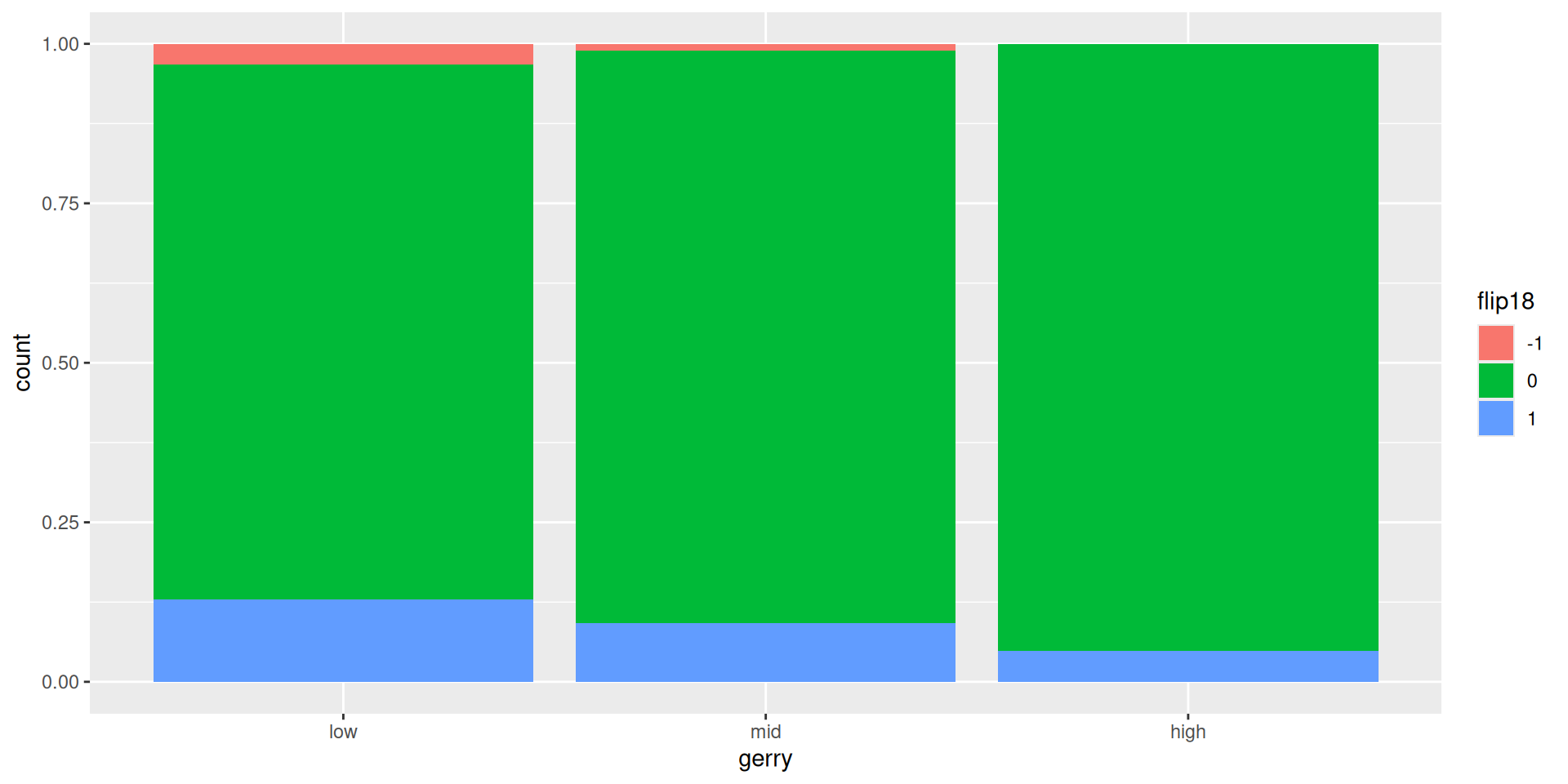
# dem18 <dbl>, gerry <fct>Revisit the plot
“Is a Congressional District more likely to be flipped to a Democratic seat if it has high prevalence of gerrymandering or low prevalence of gerrymandering?”
More about the pipe
- The pipe operator passes what comes before it into the function that comes after it as the first argument in that function.
More about the pipe
- The pipe operator passes what comes before it into the function that comes after it as the first argument in that function.
Pipe + ggplot() !!
Pipe + ggplot() !!

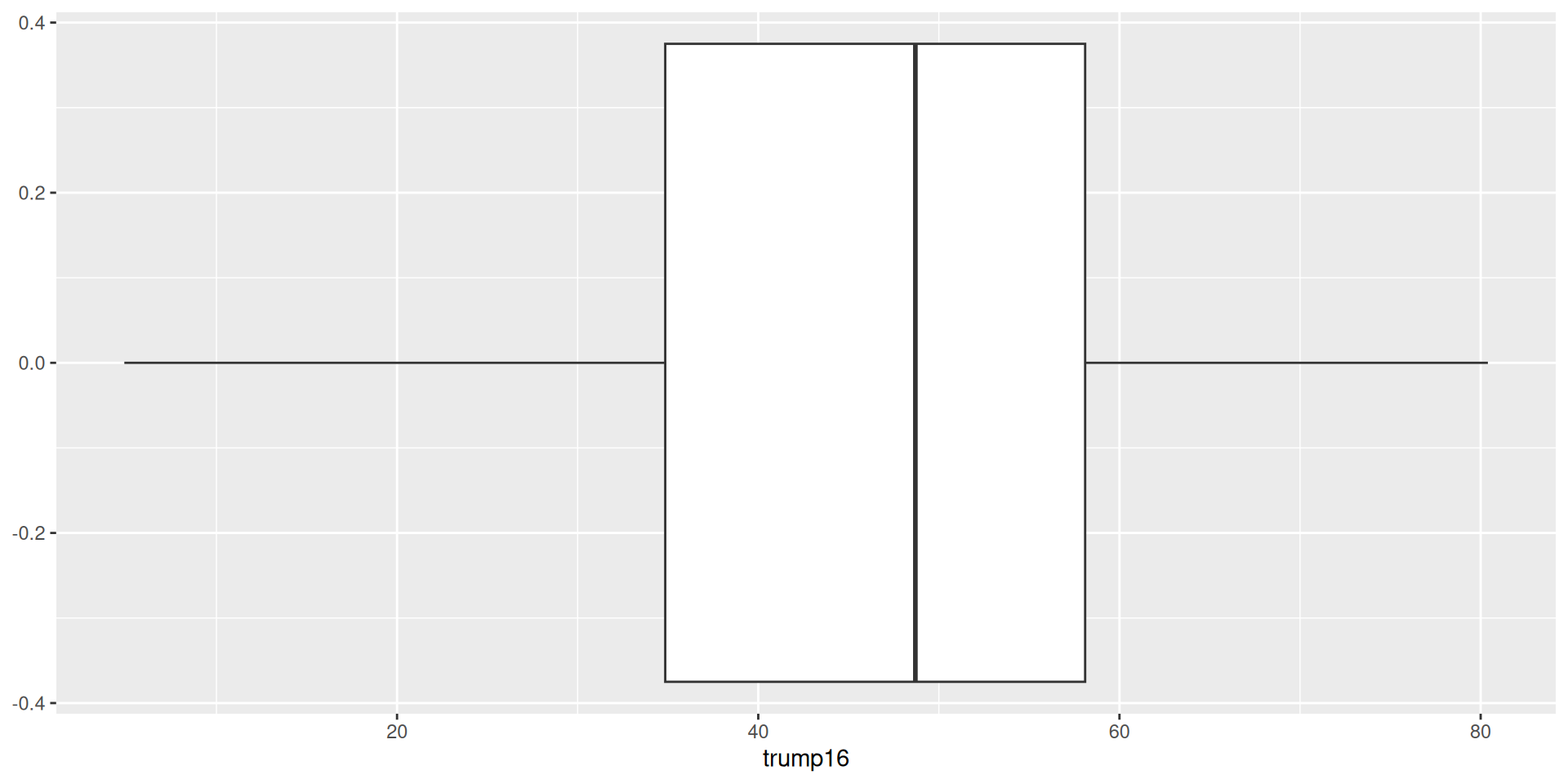
Plot + data transform
We can do data transformation immediately followed by a plot!
# A tibble: 435 × 12
   district last_name first_name party16 clinton16 trump16 dem16 state
   <chr>    <chr>     <chr>      <chr>       <dbl>   <dbl> <dbl> <chr>
 1 AK-AL    Young     Don        R            37.6    52.8     0 AK
 2 AL-01    Byrne     Bradley    R            34.1    63.5     0 AL
 3 AL-02    Roby      Martha     R            33      64.9     0 AL
 4 AL-03    Rogers    Mike D.    R            32.3    65.3     0 AL
 5 AL-04    Aderholt  Rob        R            17.4    80.4     0 AL
 6 AL-05    Brooks    Mo         R            31.3    64.7     0 AL
 7 AL-06    Palmer    Gary       R            26.1    70.8     0 AL
 8 AL-07    Sewell    Terri      D            69.8    28.6     1 AL
 9 AR-01    Crawford  Rick       R            30.2    65       0 AR
10 AR-02    Hill      French     R            41.7    52.4     0 AR
# ℹ 425 more rows
# ℹ 4 more variables: party18 <chr>, dem18 <dbl>, flip18 <dbl>,
# gerry <fct>Plot + data transform
We can do data transformation immediately followed by a plot!
# A tibble: 435 × 13
district last_name first_name party16 clinton16 trump16 dem16 state
<chr> <chr> <chr> <chr> <dbl> <dbl> <dbl> <chr>
1 AK-AL Young Don R 37.6 52.8 0 AK
2 AL-01 Byrne Bradley R 34.1 63.5 0 AL
3 AL-02 Roby Martha R 33 64.9 0 AL
4 AL-03 Rogers Mike D. R 32.3 65.3 0 AL
5 AL-04 Aderholt Rob R 17.4 80.4 0 AL
6 AL-05 Brooks Mo R 31.3 64.7 0 AL
7 AL-06 Palmer Gary R 26.1 70.8 0 AL
8 AL-07 Sewell Terri D 69.8 28.6 1 AL
9 AR-01 Crawford Rick R 30.2 65 0 AR
10 AR-02 Hill French R 41.7 52.4 0 AR
# ℹ 425 more rows
# ℹ 5 more variables: party18 <chr>, dem18 <dbl>, flip18 <dbl>,
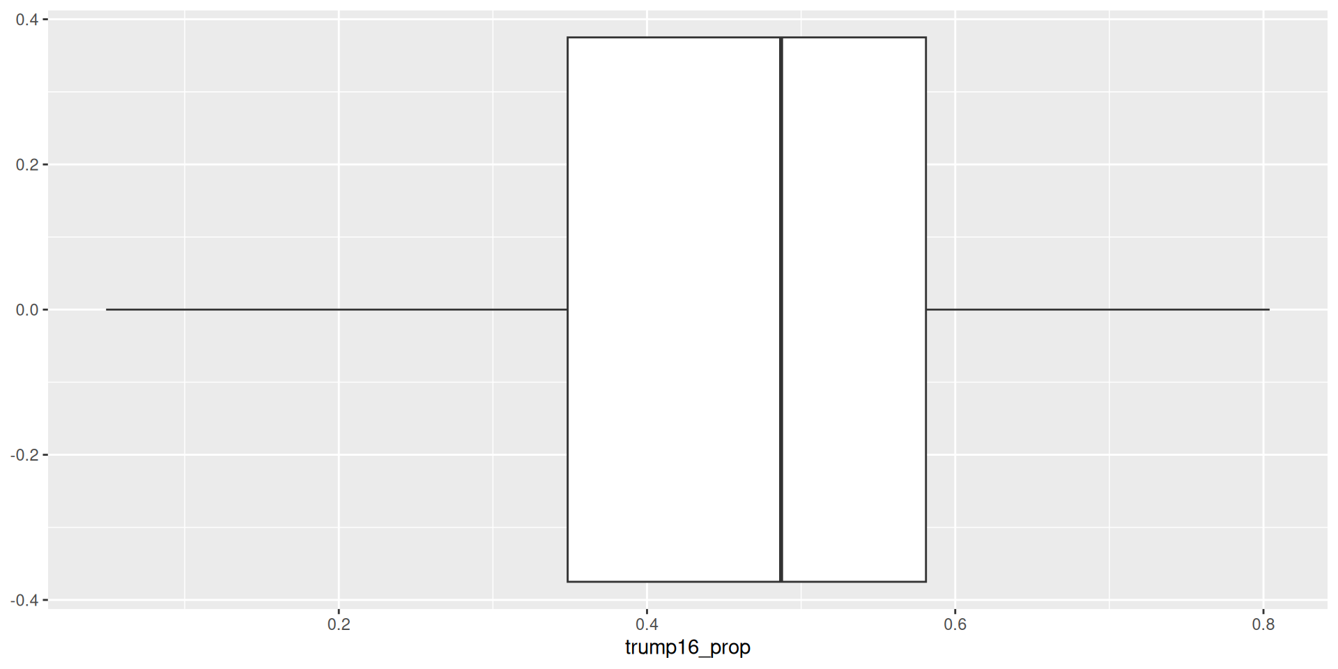
# gerry <fct>, trump16_prop <dbl>Plot + data transform
We can do data transformation immediately followed by a plot!
Plot + data transform
We can do data transformation immediately followed by a plot!
Exploratory Data Analysis
What is exploratory data analysis (EDA)??
Basically everything we have done so far
Making plots and computing summary statistics (proportions, means, IQR, etc.) to help explore the data
Generally, EDA precedes some sort of more formal statistical analysis (i.e., hypothesis testing, modeling, etc.); compare your findings from statistical analyses to key takeaways from EDA (do your findings agree? did you discern something that wasn’t visually evident (perhaps obscured by other factors not visualized)?)
You cannot make any sort of causal claim / statement from EDA alone (i.e., don’t say something like, “from this scatterplot, we see that some change in x causes some change in y)
You can observe relationships & make hypotheses!
Assignment
Let’s make a tiny data frame to use as an example:
Assignment
Do something and print to screen
Assignment
Do something, save result, overwriting original
Assignment
Do something, save result, overwriting original when you shouldn’t
Assignment
Do something, save result, overwriting original
data frame