Data Importation

Lecture 9

Katie Solarz

Duke University
STA 199 Summer 2026: Session I

May 27, 2026

Administrative Details

• Midterm next Monday!

  • Practice + some review tomorrow in class

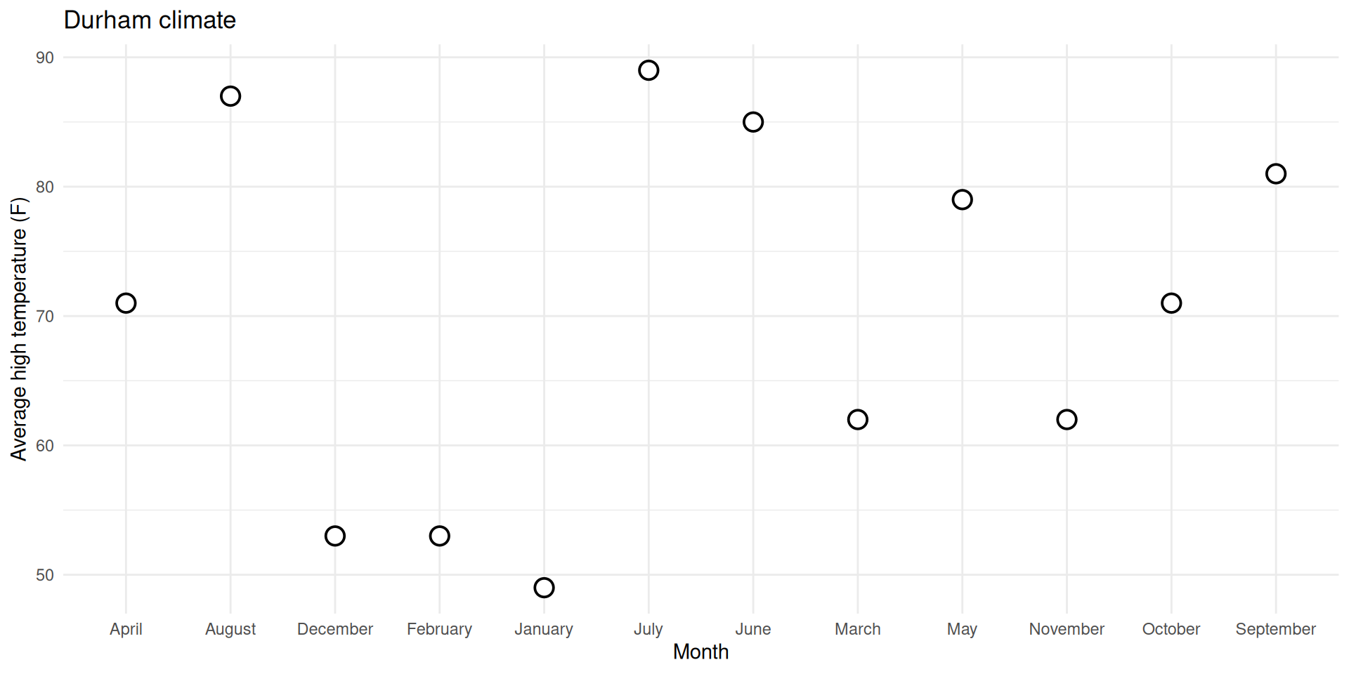
  • Practice questions for both the multiple choice & live coding portions of the exam will be posted tomorrow!

  • I will post solutions to the practice questions by Saturday morning

• Lab 3 after lecture tomorrow

  • This will be a shorter than usual lab & is meant to serve as a recap of all we’ve learned so far (aka, helpful exam prep!)

  • Reminder: Lab 3 will be due by 12:00pm (noon) on Sunday; there will be no late window for this lab assignment

  • Solutions will posted to the website promptly thereafter

Administrative Details

• Project work begins next week! More details on what the project is tomorrow :)

  • Since the midterm takes place during both of the formal lecture and lab timeslots next Monday, lecture time next Tuesday (9:30am - 10:45am) will function as a lab meeting

  • Both lab sessions next week (T, Th) will be dedicated worktime

  • You will receive your team assignments (2 groups of 3, 2 groups of 4) in lab next Tuesday

  • As a reminder, projects are completed in groups BUT grades are individual; your final project grade may ultimately differ from your teammates’ if there is unequal participation

  • Participation is measured by 1) lab attendance on project work days; 2) commit history in project repos on GitHub; 3) peer review forms

Back to AE-08

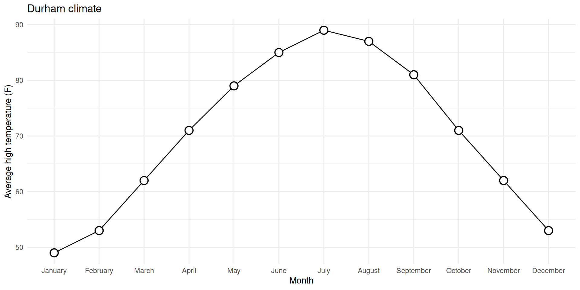
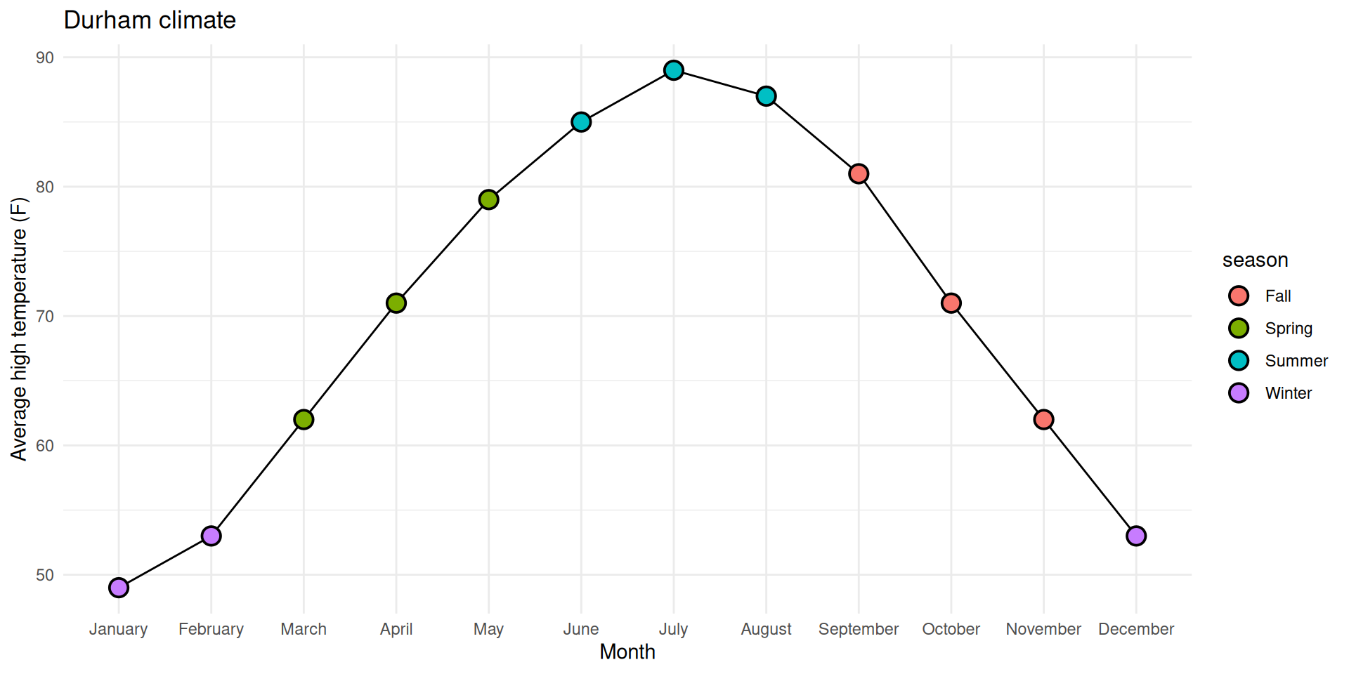
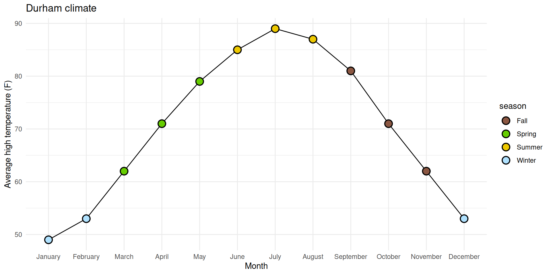
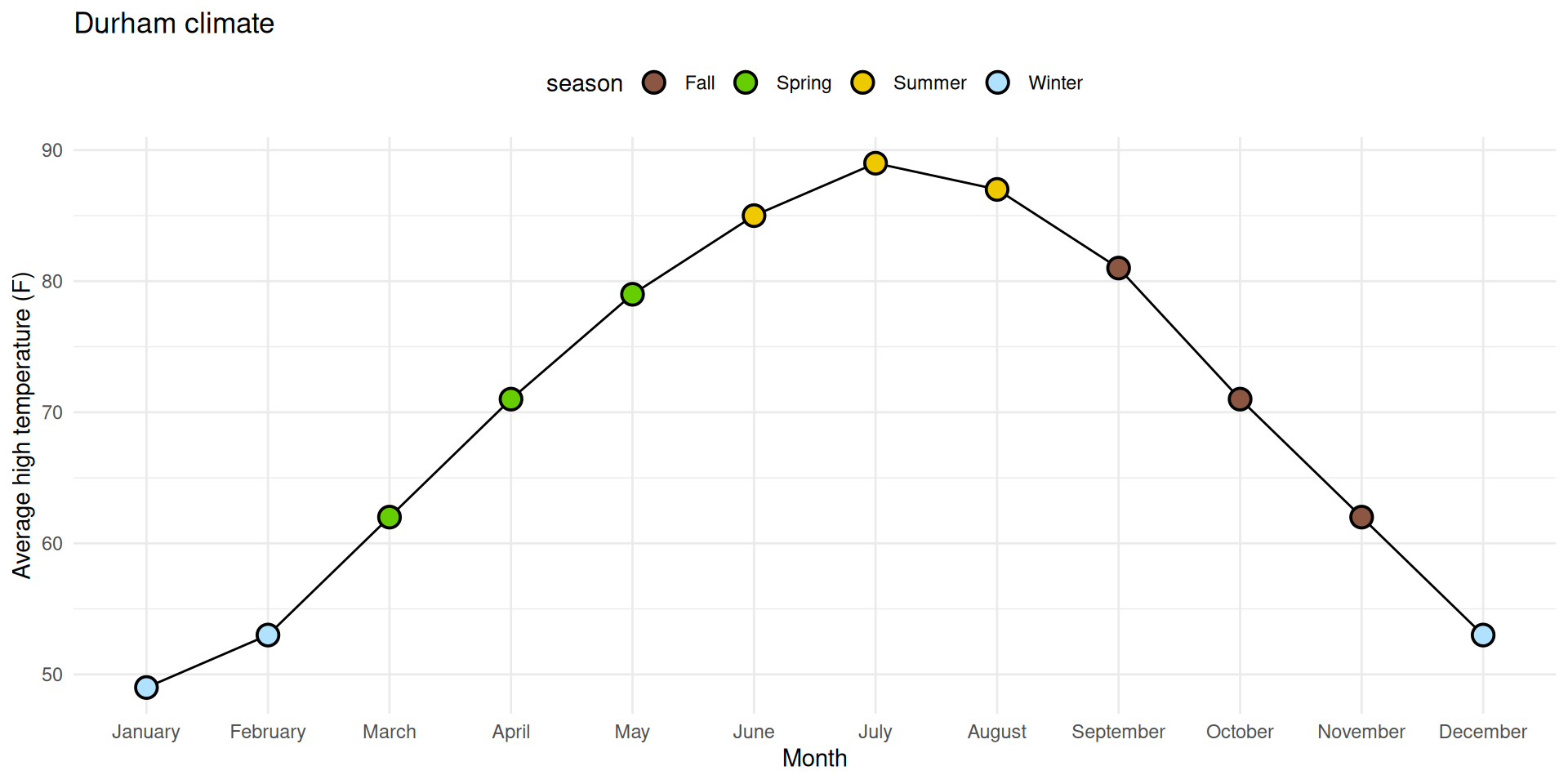
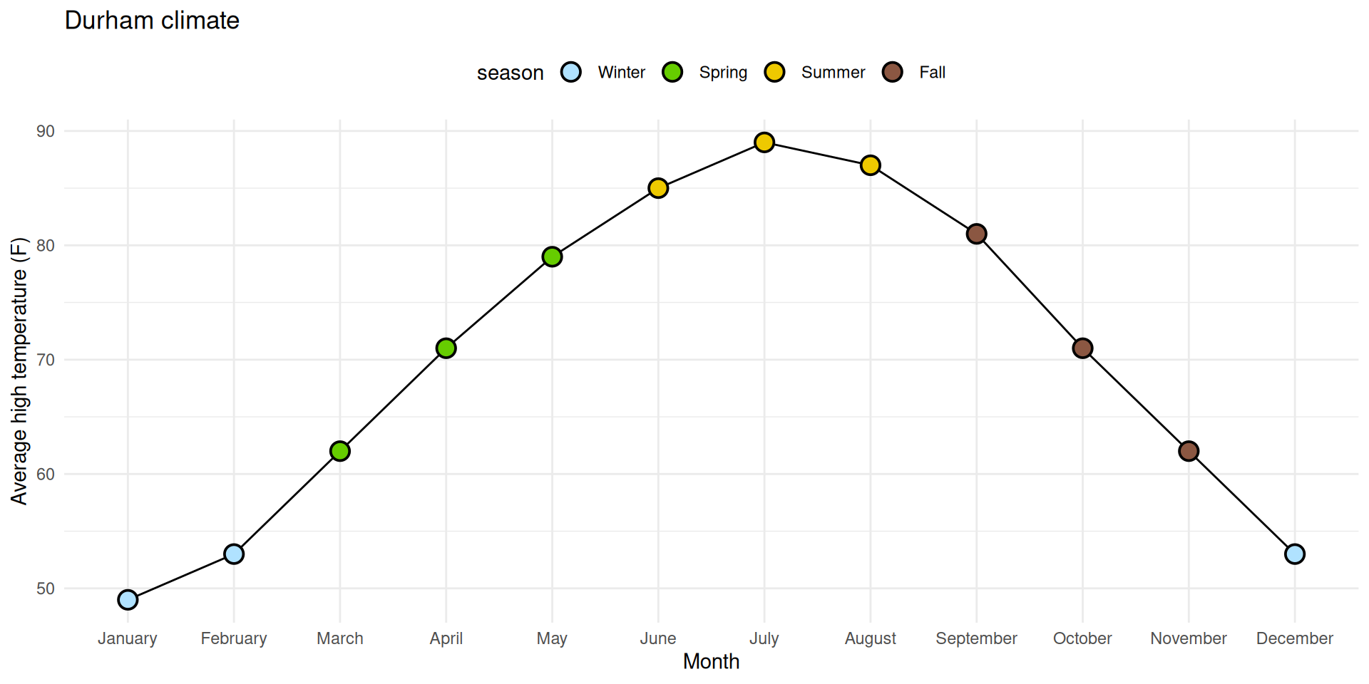
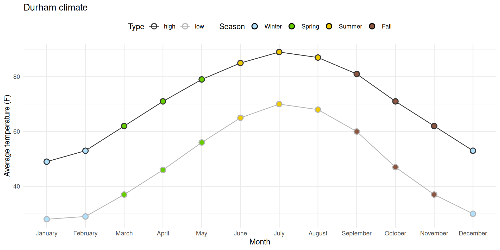
Task 1: Prettifying the plot from ae-08

ggplot(
  durham_climate, 
  aes(x = month, y = avg_high_f, group = 1)
  ) +
  geom_line() +
  geom_point(
    shape = "circle filled", size = 4,
    color = "black", fill = "white", stroke = 1
  ) +
  labs(
    x = "Month",
    y = "Average high temperature (F)",
    title = "Durham climate"
  ) + 
  theme_minimal()

Things to change

1. ✅ Reorder the months chronologically;
2. ✅ Fill the circles with season-specific colors;
3. ⬜ Add a legend for these colors to the top of the plot;
4. ⬜ Make sure the legend is ordered chronologically by season.

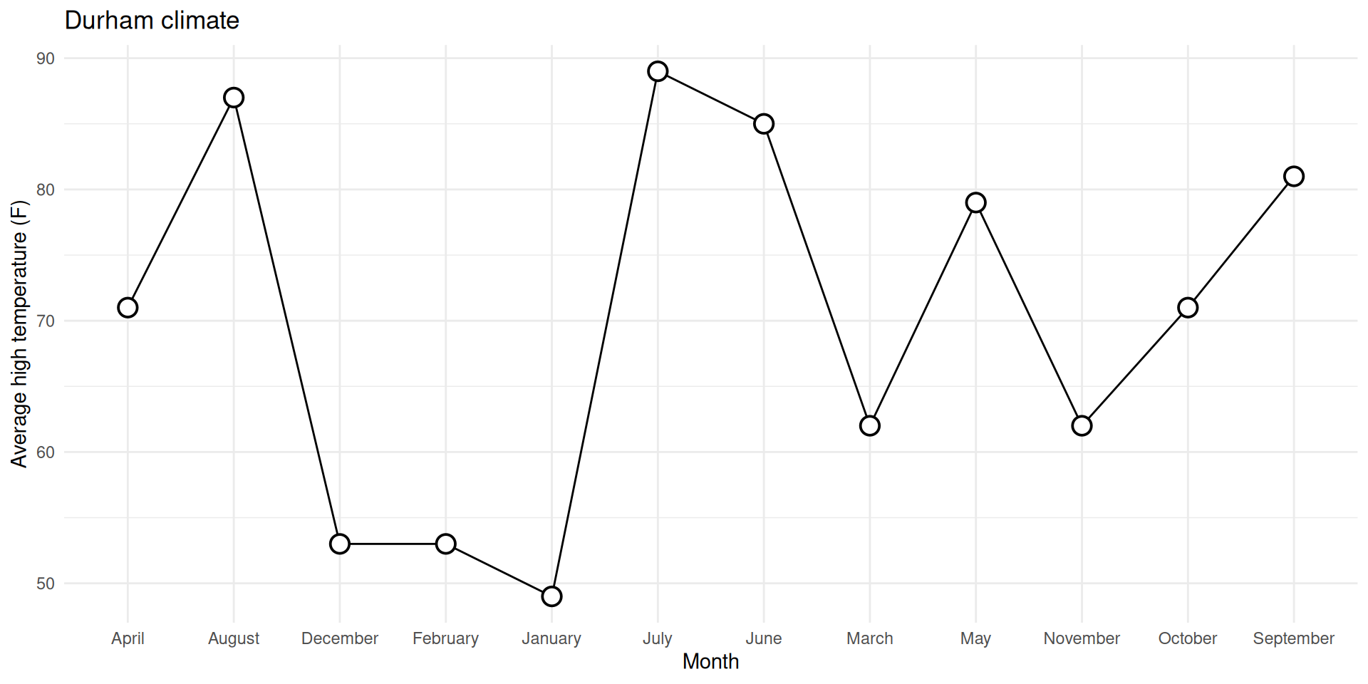
0. Why group = 1?

With it:

ggplot(
  durham_climate, 
  aes(x = month, y = avg_high_f, group = 1)
  ) +
  geom_line() +
  geom_point(
    shape = "circle filled", size = 4,
    color = "black", fill = "white", stroke = 1
  ) +
  labs(
    x = "Month",
    y = "Average high temperature (F)",
    title = "Durham climate"
  ) +
  theme_minimal()

0. Why group = 1?

Without it (even though I have geom_line!):

ggplot(
  durham_climate, 
  aes(x = month, y = avg_high_f)
  ) +
  geom_line() +
  geom_point(
    shape = "circle filled", size = 4,
    color = "black", fill = "white", stroke = 1
  ) +
  labs(
    x = "Month",
    y = "Average high temperature (F)",
    title = "Durham climate"
  ) +
  theme_minimal()

`geom_line()`: Each group consists of only one observation.
ℹ Do you need to adjust the group aesthetic?

0. Why group = 1?

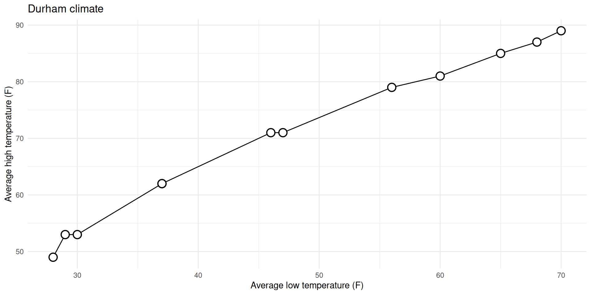
Don’t need group = argument for numerical vs numerical:

ggplot(
  durham_climate, 
  aes(x = avg_low_f, y = avg_high_f)
  ) +
  geom_line() +
  geom_point(
    shape = "circle filled", size = 4,
    color = "black", fill = "white", stroke = 1
  ) +
  labs(
    x = "Average low temperature (F)",
    y = "Average high temperature (F)",
    title = "Durham climate"
  ) +
  theme_minimal()

0. Why group = 1?

Do need group = argument for categorical vs numerical:

ggplot(
  durham_climate, 
  aes(x = month, y = avg_high_f, group = 1)
  ) +
  geom_line() +
  geom_point(
    shape = "circle filled", size = 4,
    color = "black", fill = "white", stroke = 1
  ) +
  labs(
    x = "Month",
    y = "Average high temperature (F)",
    title = "Durham climate"
  ) +
  theme_minimal()

1. Reorder the months chronologically

durham_climate |>
  mutate(
    month = fct_relevel(month, month.name)
  ) |>
  ggplot(
    aes(x = month, y = avg_high_f, group = 1)
  ) +
  geom_line() +
  geom_point(
    shape = "circle filled", size = 4,
    color = "black", fill = "white", stroke = 1
  ) +
  labs(
    x = "Month",
    y = "Average high temperature (F)",
    title = "Durham climate"
  ) +
  theme_minimal()

2. Fill the circles with season-specific colors

durham_climate |>
  mutate(
    month = fct_relevel(month, month.name),
    season = case_when(
      month %in% c("December", "January", "February") ~ "Winter",
      month %in% c("March", "April", "May") ~ "Spring",
      month %in% c("June", "July", "August") ~ "Summer",
      month %in% c("September", "October", "November") ~ "Fall",
    )
  ) |>
  ggplot(
    aes(x = month, y = avg_high_f, group = 1)
    ) +
  geom_line() +
  geom_point(
    aes(fill = season),
    shape = "circle filled", size = 4,
    color = "black", stroke = 1
  ) +
  labs(
    x = "Month",
    y = "Average high temperature (F)",
    title = "Durham climate"
  ) +
  theme_minimal()

2.5 Let’s choose different-than-default season-specific colors

durham_climate |>
  mutate(
    month = fct_relevel(month, month.name),
    season = case_when(
      month %in% c("December", "January", "February") ~ "Winter",
      month %in% c("March", "April", "May") ~ "Spring",
      month %in% c("June", "July", "August") ~ "Summer",
      month %in% c("September", "October", "November") ~ "Fall",
    )
  ) |>
  ggplot(
    aes(x = month, y = avg_high_f, group = 1)
    ) +
  geom_line() +
  geom_point(
    aes(fill = season),
    shape = "circle filled", size = 4,
    color = "black", stroke = 1
  ) +
  scale_fill_manual(
    values = c(
      "Winter" = "lightskyblue1",
      "Spring" = "chartreuse3",
      "Summer" = "gold2",
      "Fall" = "lightsalmon4"
    )
  ) + 
  labs(
    x = "Month",
    y = "Average high temperature (F)",
    title = "Durham climate"
  ) +
  theme_minimal()

3. Add legend for season to top of plot

durham_climate |>
  mutate(
    month = fct_relevel(month, month.name),
    season = case_when(
      month %in% c("December", "January", "February") ~ "Winter",
      month %in% c("March", "April", "May") ~ "Spring",
      month %in% c("June", "July", "August") ~ "Summer",
      month %in% c("September", "October", "November") ~ "Fall",
    )
  ) |>
  ggplot(
    aes(x = month, y = avg_high_f, group = 1)
    ) +
  geom_line() +
  geom_point(
    aes(fill = season),
    shape = "circle filled", size = 4,
    color = "black", stroke = 1
  ) +
  scale_fill_manual(
    values = c(
      "Winter" = "lightskyblue1",
      "Spring" = "chartreuse3",
      "Summer" = "gold2",
      "Fall" = "lightsalmon4"
    )
  ) + 
  labs(
    x = "Month",
    y = "Average high temperature (F)",
    title = "Durham climate"
  ) +
  theme_minimal() + 
  theme(legend.position = "top")

4. Order legend chronologically

durham_climate |>
  mutate(
    month = fct_relevel(month, month.name),
    season = case_when(
      month %in% c("December", "January", "February") ~ "Winter",
      month %in% c("March", "April", "May") ~ "Spring",
      month %in% c("June", "July", "August") ~ "Summer",
      month %in% c("September", "October", "November") ~ "Fall",
    ),
    season = fct_relevel(season, "Winter", "Spring", "Summer", "Fall")
  ) |>
  ggplot(
    aes(x = month, y = avg_high_f, group = 1)
    ) +
  geom_line() +
  geom_point(
    aes(fill = season),
    shape = "circle filled", size = 4,
    color = "black", stroke = 1
  ) +
  scale_fill_manual(
    values = c(
      "Winter" = "lightskyblue1",
      "Spring" = "chartreuse3",
      "Summer" = "gold2",
      "Fall" = "lightsalmon4"
    )
  ) + 
  labs(
    x = "Month",
    y = "Average high temperature (F)",
    title = "Durham climate"
  ) +
  theme_minimal() + 
  theme(legend.position = "top")

Task 2: pivot to replicate this…

Give it a shot in your ae-08 .qmd file… you can ignore the prettification we walked through for now.

Let’s zoom out for a second

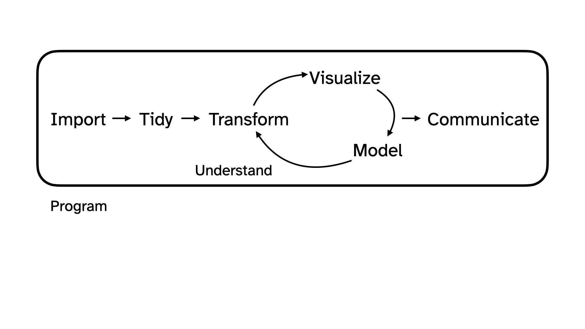
Data science and statistical thinking

Before Midterm 1…

• Data science: the real-world art of transforming messy, imperfect, incomplete data into knowledge;

After Midterm 1…

• Statistics: the mathematical discipline of quantifying our uncertainty about that knowledge.

Data science

Data science

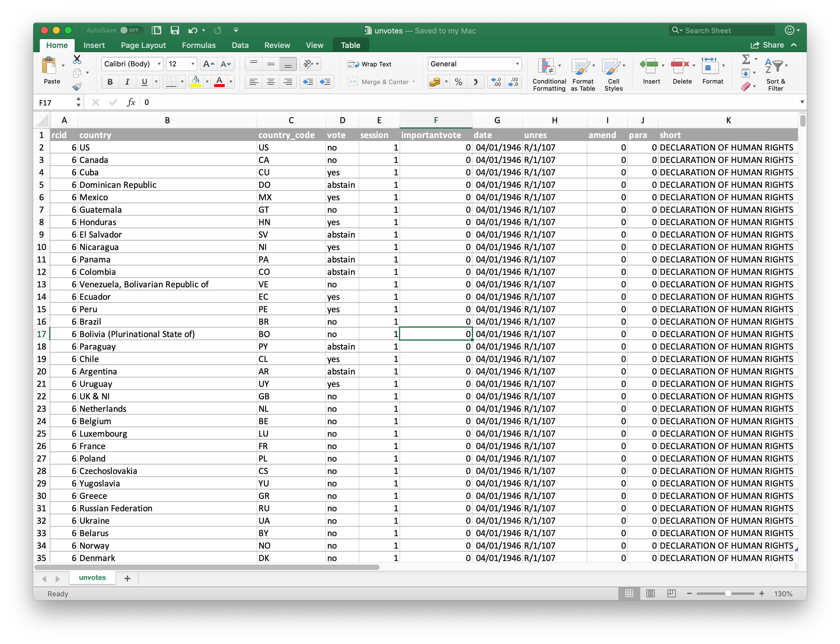
1. Collection: we won’t seriously study data collection (take an experimental design class if you are interested!); we will discuss data importation methods today

• for the purposes of this class: accessing package data (library(); df <- library::df), data importation (read_csv, read_xlsx, read_xls)
• in reality…: web-scraping, domain-specific issues of measurement, survey design, experimental design, etc.

Data science

1. Collection: we won’t seriously study data collection; we will discuss data importation methods today

2. Preparation: cleaning, wrangling, and otherwise tidying the data so we can actually work with it.

• keywords: mutate, fct_relevel, pivot_*, *_join

Data science

1. Collection: we won’t seriously study data collection; we will discuss data importation methods today

2. Preparation: cleaning, wrangling, and otherwise tidying the data so we can actually work with it.

3. Analysis: finally, transform the data into knowledge…

• visual summaries: ggplot, geom_*, etc.
• numerical summaries: summarize, group_by, count, mean, median, sd, quantile, IQR, cor, etc.
• The visualizations and the summaries should complement one another!

Reading data into R

Package data

• When data is neatly stored in a package, such as tidyverse, loading the package loads the dataset; you can explicitly save a packaged df to your RStudio environment by running df <- library::df

• Most often, this is not the case

Reading in rectangular data

Reading rectangular data

• Using readr: (in tidyverse)
  • Most commonly: read_csv() - file saved as .csv
  • Maybe also: read_tsv(), read_delim(), etc - other file formats

• Using readxl:
  • read_excel() - R determines file type for you
  • read_xls(), read_xlsx() - use if you know whether you have a .xls or .xlsx file

• Using googlesheets4: read_sheet() – we haven’t covered this in the videos, but might be useful for your projects

  • Fun fact: The “Schedule” page on the course website pulls information from an underlying Google sheets file

Using read_csv()

Generally, the format is:

df_name <- read_csv("path_to_file_name.csv")

Path to file

For example, recall we worked with durham-climate.csv in AE08. Where is durham-climate.csv?

When in our AE repo, we read in the data with the following code:

durham_climate <- read_csv("data/durham-climate.csv")

Path to file

• use / to separate folder(s) + file names; file path in quotes

• Answer: read_csv("data/durham-climate.csv")

Why not include ae-kgsolarz?

Where is durham-climate.csv?

We can also write files!

This allows us to save data for later usage, share data outside of R, etc.

Using write_csv():

write_csv(r_df_name, "path_to_file.csv")

Application exercise

Goal 1.1: Reading and writing CSV files

• Read a CSV file with tidy data

• Split it into subsets based on features of the data

• Write out subsets as CSV files

Goal 1.2: Practice - Case When

• case_when() is similar to if_else(), but allows multiple cases
• case_when() is often used within mutate() to create a new column

df |>
  mutate(new_var = case_when(
    condition_1 ~ result_1,
    condition_2 ~ result_2,
    condition_3 ~ result_3,
    ...,
    .default = default_result
  ))

An aside - If Else

• case_when() is similar to if_else(), but if_else() only allows for 2 cases / conditions

• Long story short… use if_else() if you are only considering 2 cases / conditions; for > 2 conditions, use case_when()

• In words, we’d read the code below as: “If logical_1 evaluates to TRUE (i.e., this condition is met), then choose result_1; else (i.e., this condition is not met), choose result 2

df |>
  mutate(new_var = if_else(logical_1, result_1, result_2))

## create a new column, "is_december" with a value 1 if the month is December and a value 0 otherwise

durham_climate |>
  mutate(is_december = if_else(month == "December", 1, 0))

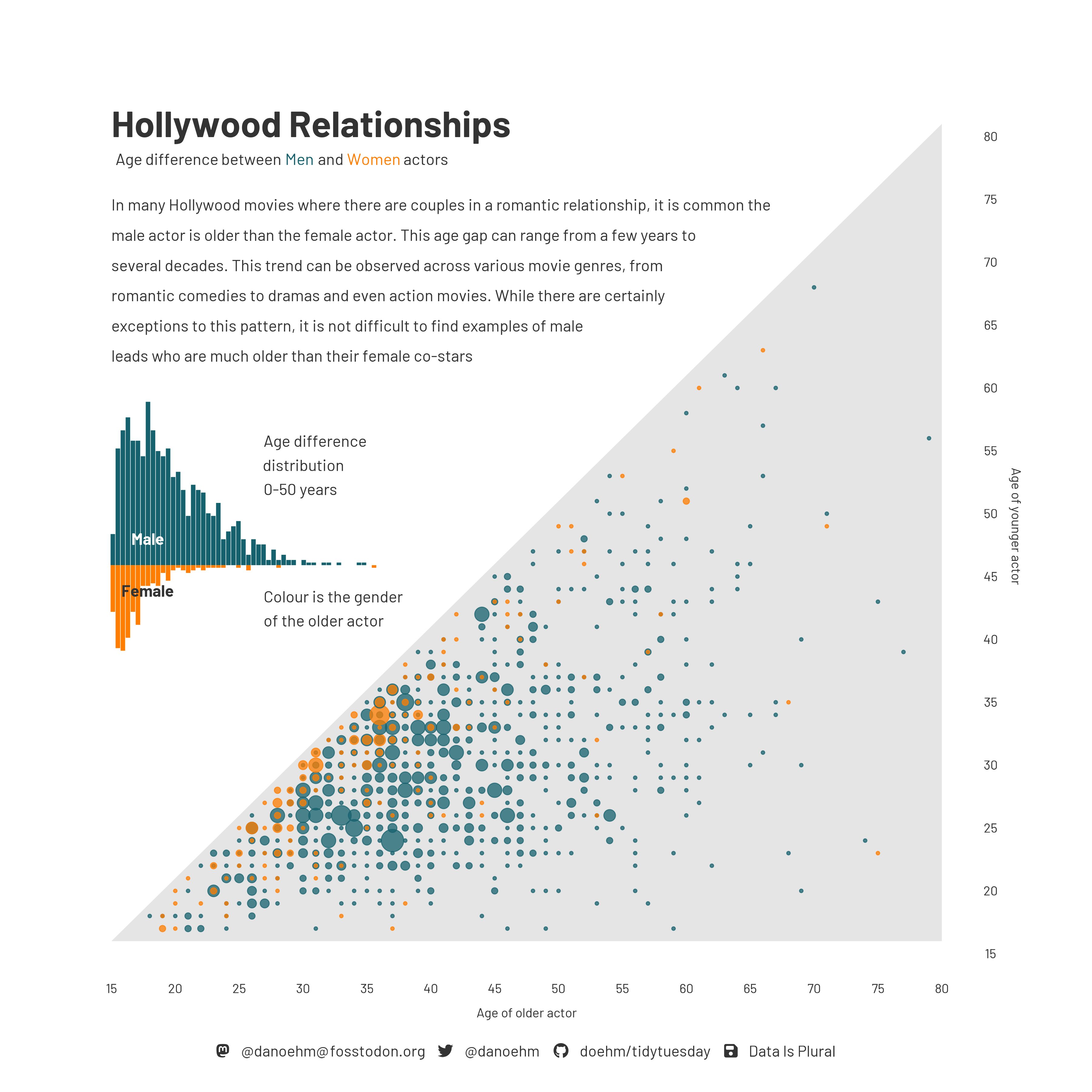
Age gap in Hollywood relationships

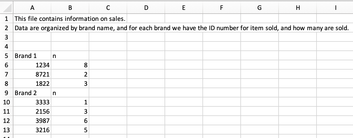
Goal 2.1: Reading Excel files & non-tidy data

• Read an Excel file with non-tidy data

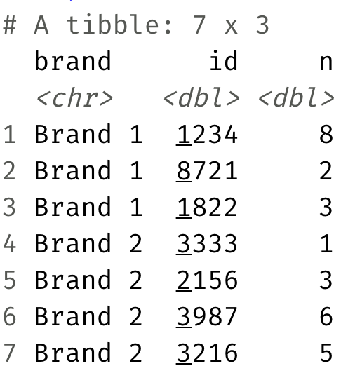
• Tidy it up!

Goal 2.2: String Functions

We’ve seen lots of functions that deal with numeric data (mean, median, sum, etc.) - what about characters?

• stringr is a tidyverse package with lots of functions for dealing with character strings

• today: str_detect in stringr

Goal 2.2: String Functions

• str_detect() identifies if a character / sequence of characters is a substring within a longer string

• useful in cases when you need to check some condition, for example:

  • in a filter()

  • in an if_else() or case_when()

Goal 2.2: String Functions

• str_detect() identifies if a character / sequence of characters is a substring within a longer string

• useful in cases when you need to check some condition, for example:

  • in a filter()

  • in an if_else() or case_when()

example: which classes in a list are in the stats department?

classes <- c("sta199", "dance122", "math185", "sta240", "pubpol202")
str_detect(classes, "sta")

[1]  TRUE FALSE FALSE  TRUE FALSE

Goal 2.2: String Functions

General form:

str_detect(character_var, "word_to_detect")

Sales data

Are these data tidy? Why or why not?

Sales data

What data tidying must be done to go from the original, non-tidy data to the below tidy version of these data?