The Language of Models

Lecture 12

Katie Solarz

Duke University
STA 199 Summer 2026: Session I

June 3, 2026

While you wait…

• Go to your ae project in RStudio.

• Make sure all of your changes up to this point are committed and pushed, i.e., there’s nothing left in your Git pane.

• Click Pull to get today’s application exercise file: ae-12-modeling-fish.qmd.

• Wait till the you’re prompted to work on the application exercise during class before editing the file.

Midterm is done!

This course is officially halfway over 💔🍾

Modeling

Before:

• Plotting and summary statistics

• Useful, but… a little subjective?

Now:

• Learn statistical tools for quantifying relationships
  • Describing relationships
  • Prediction and classification
  • Uncertainty quantification

Today’s Agenda

• What is a model?
• Why do we model?
• What is correlation?

Prediction / classification

Let’s drive a Tesla!

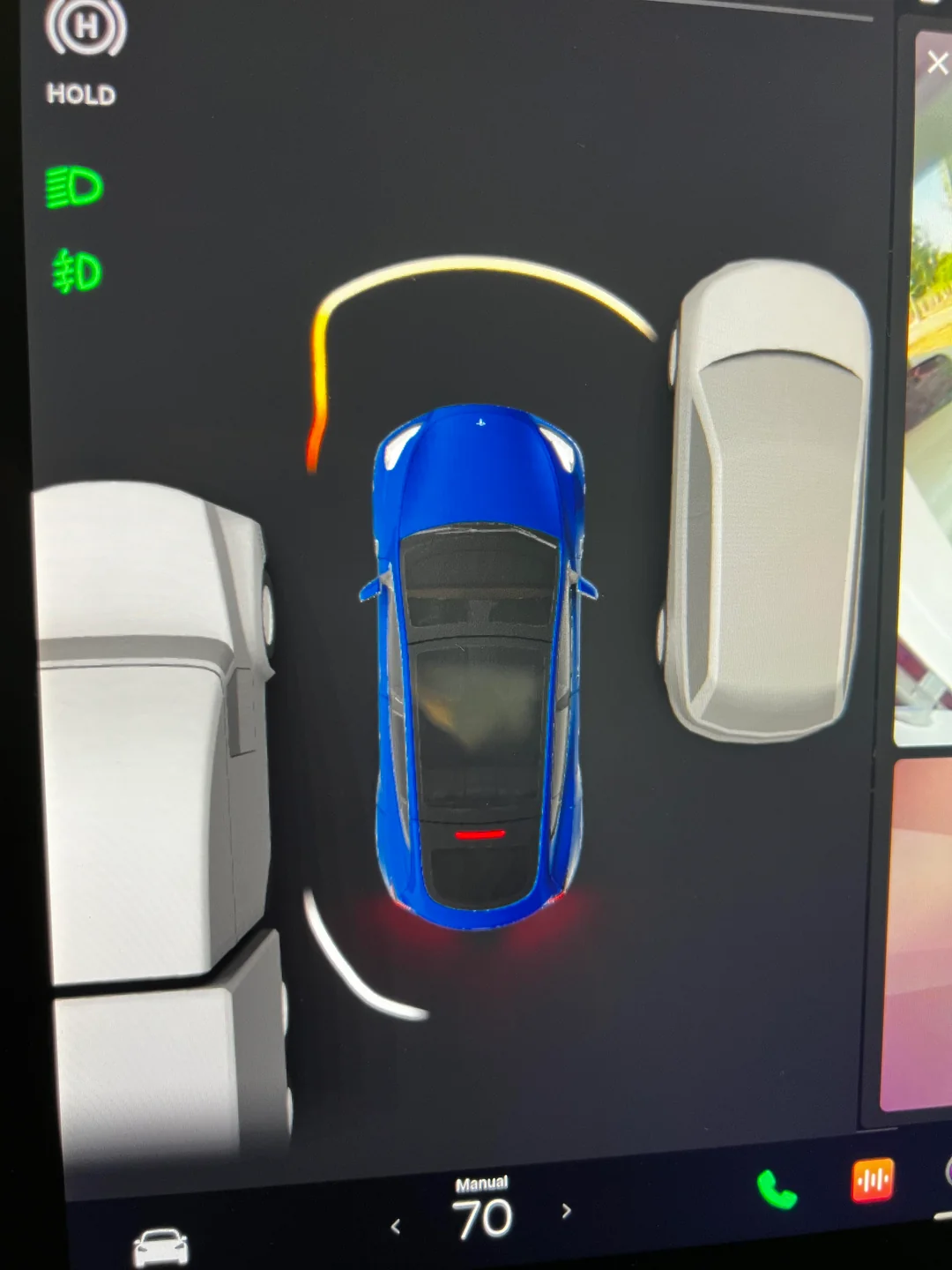
Semi or garage?

i love how Tesla thinks the wall in my garage is a semi. 😅

Source: Reddit

Semi or garage?

New owner here. Just parked in my garage. Tesla thinks I crashed onto a semi.

Source: Reddit

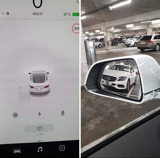
Car or trash?

Tesla calls Mercedes trash

Source: Reddit

Description

Leisure, commute, physical activity and BP

Relation Between Leisure Time, Commuting, and Occupational Physical Activity With Blood Pressure in 125,402 Adults: The Lifelines Cohort

Byambasukh, Oyuntugs, Harold Snieder, and Eva Corpeleijn. “Relation between leisure time, commuting, and occupational physical activity with blood pressure in 125 402 adults: the lifelines cohort.” Journal of the American Heart Association 9.4 (2020): e014313.

Leisure, commute, physical activity and BP

Goal: To investigate the associations of different domains of daily‐life physical activity, such as commuting, leisure‐time, and occupational, with BP level and the risk of having hypertension.

Leisure, commute, physical activity and BP

Goal: To investigate the associations of different domains of daily-life physical activity, such as commuting, leisure-time, and occupational, with BP level and the risk of having hypertension.

Methods and Results: In the population-based Lifelines cohort (N=125,402), MVPA was assessed by the Short Questionnaire to Assess Health-Enhancing Physical Activity, a validated questionnaire in different domains such as commuting, leisure-time, and occupational PA.

Leisure, commute, physical activity and BP

Goal: To investigate the associations of different domains of daily-life physical activity, such as commuting, leisure-time, and occupational, with BP level and the risk of having hypertension.

Methods and Results: In the population-based Lifelines cohort (N=125,402), MVPA was assessed by the Short Questionnaire to Assess Health-Enhancing Physical Activity, a validated questionnaire in different domains such as commuting, leisure-time, and occupational PA. Commuting-and-leisure-time MVPA was associated with BP in a dose-dependent manner.

Leisure, commute, physical activity and BP

Goal: To investigate the associations of different domains of daily-life physical activity, such as commuting, leisure-time, and occupational, with BP level and the risk of having hypertension.

Methods and Results: In the population-based Lifelines cohort (N=125,402), MVPA was assessed by the Short Questionnaire to Assess Health-Enhancing Physical Activity, a validated questionnaire in different domains such as commuting, leisure-time, and occupational PA. Commuting-and-leisure-time MVPA was associated with BP in a dose-dependent manner. β Coefficients (95% CI) from linear regression analyses were −1.64 (−2.03 to −1.24), −2.29 (−2.68 to −1.90), and −2.90 (−3.29 to −2.50) mm Hg systolic BP for the low, middle, and highest tertile of MVPA compared with “No MVPA” as the reference group after adjusting for age, sex, education, smoking and alcohol use. Further adjustment for body mass index attenuated the associations by 30% to 50%, but more MVPA remained significantly associated with lower BP and lower risk of hypertension. This association was age dependent. β Coefficients (95% CI) for the highest tertiles of commuting-and-leisure-time MVPA were −1.67 (−2.20 to −1.15), −3.39 (−3.94 to −2.82) and −4.64 (−6.15 to −3.14) mm Hg systolic BP in adults <40, 40 to 60, and >60 years, respectively.

Leisure, commute, physical activity and BP

Goal: To investigate the associations of different domains of daily-life physical activity, such as commuting, leisure-time, and occupational, with BP level and the risk of having hypertension.

Methods and Results: In the population-based Lifelines cohort (N=125,402), MVPA was assessed by the Short Questionnaire to Assess Health-Enhancing Physical Activity, a validated questionnaire in different domains such as commuting, leisure-time, and occupational PA. Commuting-and-leisure-time MVPA was associated with BP in a dose-dependent manner. β Coefficients (95% CI) from linear regression analyses were −1.64 (−2.03 to −1.24), −2.29 (−2.68 to −1.90), and −2.90 (−3.29 to −2.50) mm Hg systolic BP for the low, middle, and highest tertile of MVPA compared with “No MVPA” as the reference group after adjusting for age, sex, education, smoking and alcohol use. Further adjustment for body mass index attenuated the associations by 30% to 50%, but more MVPA remained significantly associated with lower BP and lower risk of hypertension. This association was age dependent. β Coefficients (95% CI) for the highest tertiles of commuting-and-leisure-time MVPA were −1.67 (−2.20 to −1.15), −3.39 (−3.94 to −2.82) and −4.64 (−6.15 to −3.14) mm Hg systolic BP in adults <40, 40 to 60, and >60 years, respectively.

Conclusions: Higher commuting and leisure-time but not occupational MVPA were significantly associated with lower BP and lower hypertension risk at all ages, but these associations were stronger in older adults.

Let’s go

Modeling cars

• What is the relationship between cars’ weights and their gas mileage?
• What is your best guess for a car’s MPG that weighs 4,500 pounds?

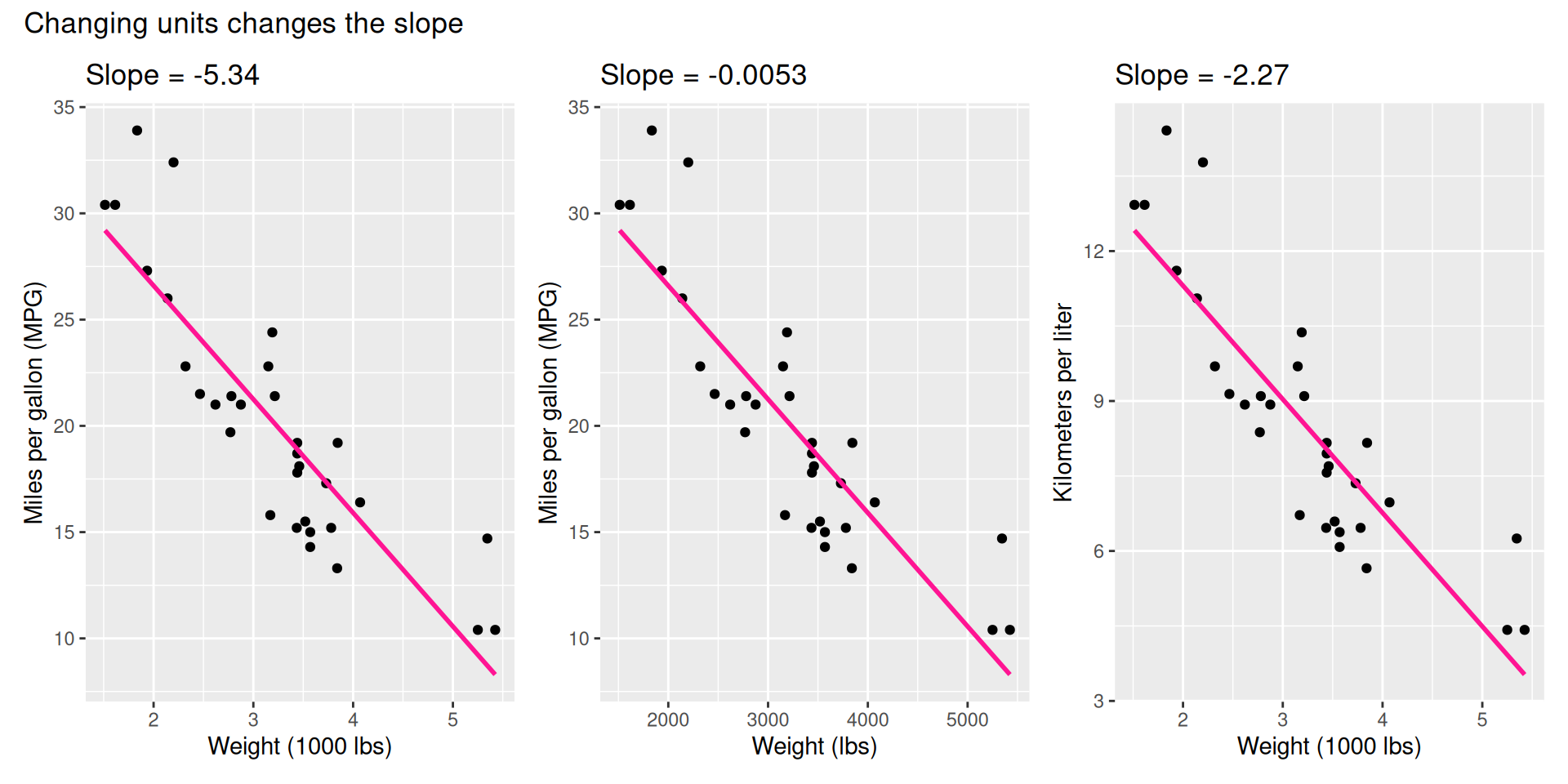
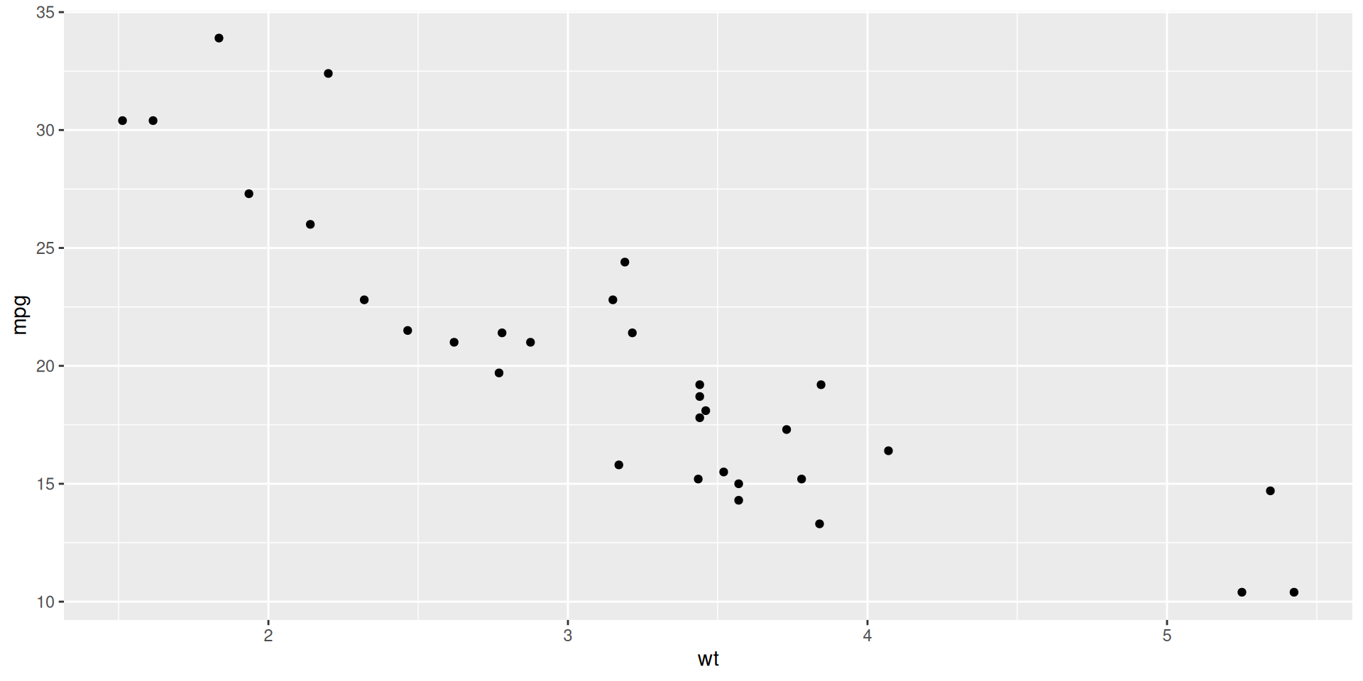
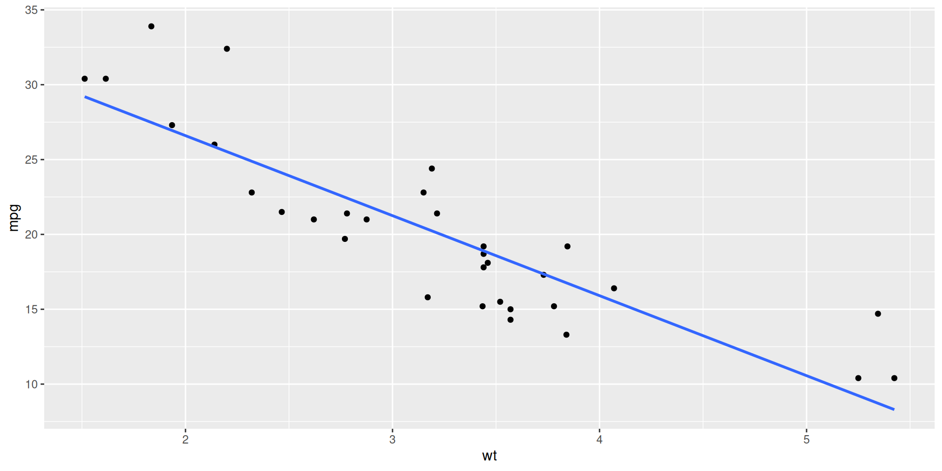
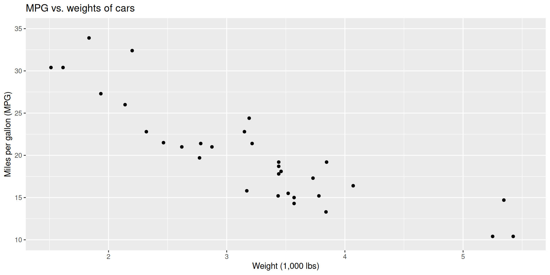
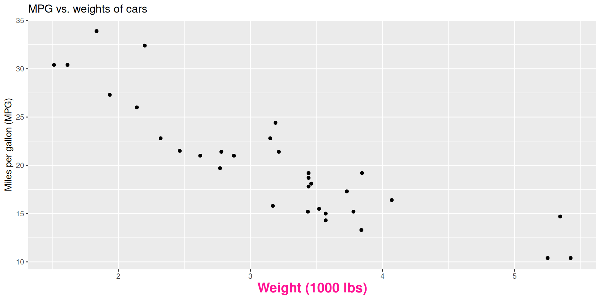
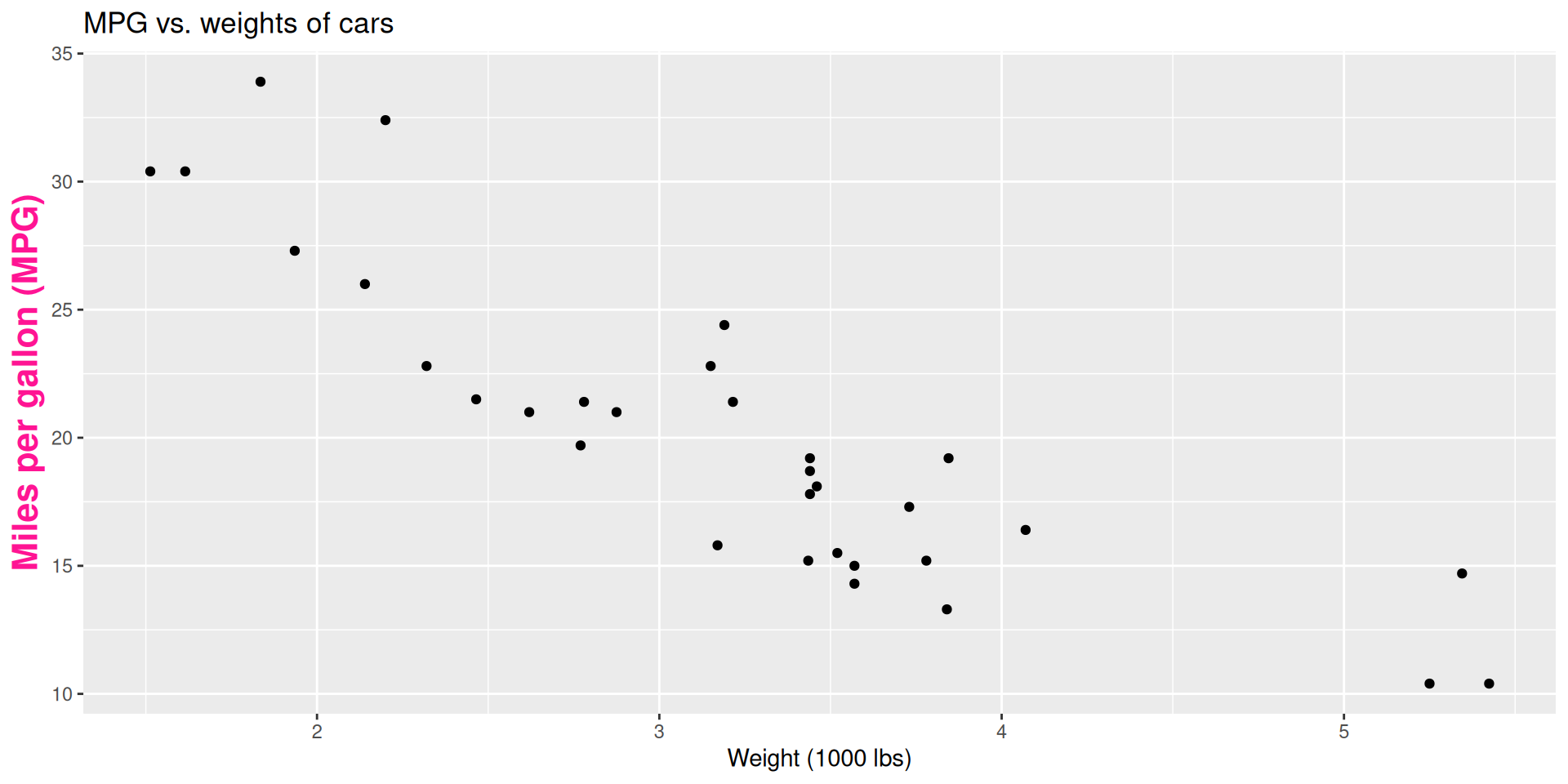
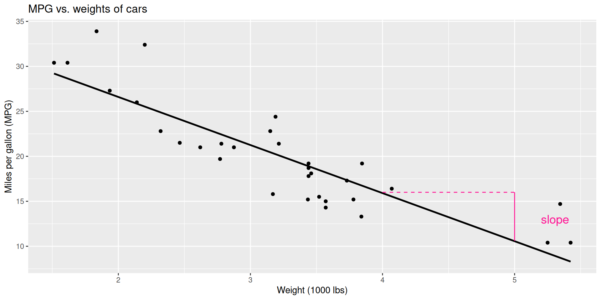
Modeling cars

Describe: What is the relationship between cars’ weights and their gas mileage?

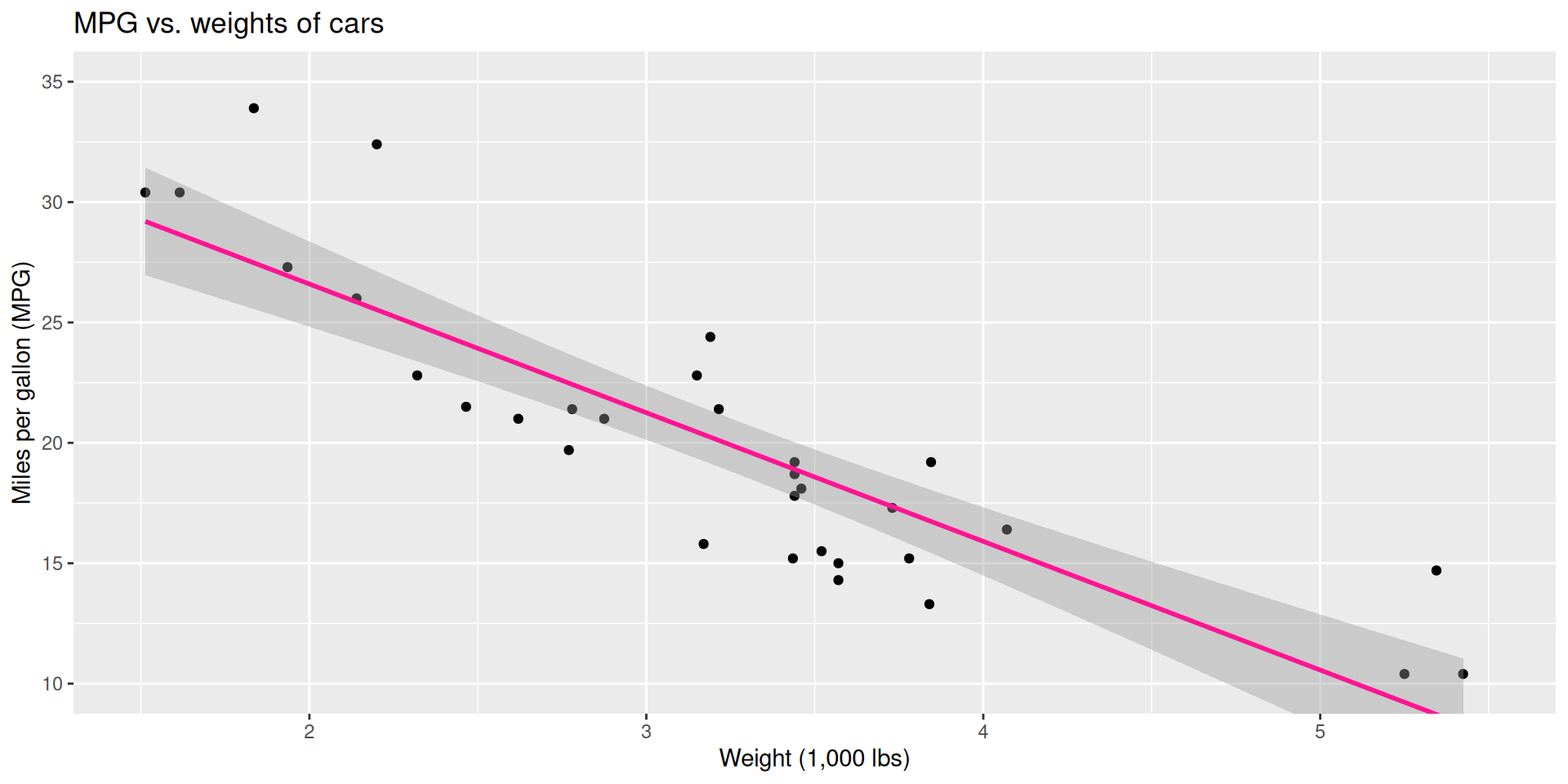
Modeling cars

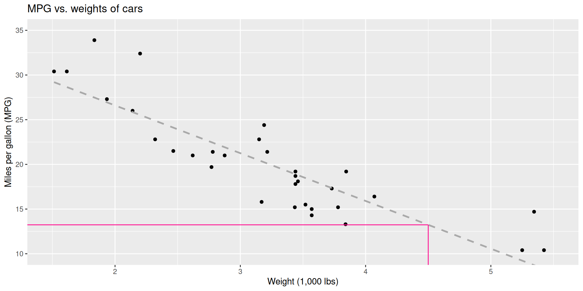
Predict: What is your best guess for a car’s MPG that weighs 4,500 pounds?

Modeling

• We use statistical models to explain the relationship between variables and to make predictions
• For now, we will focus on linear models (but there are many many other types of models too!)

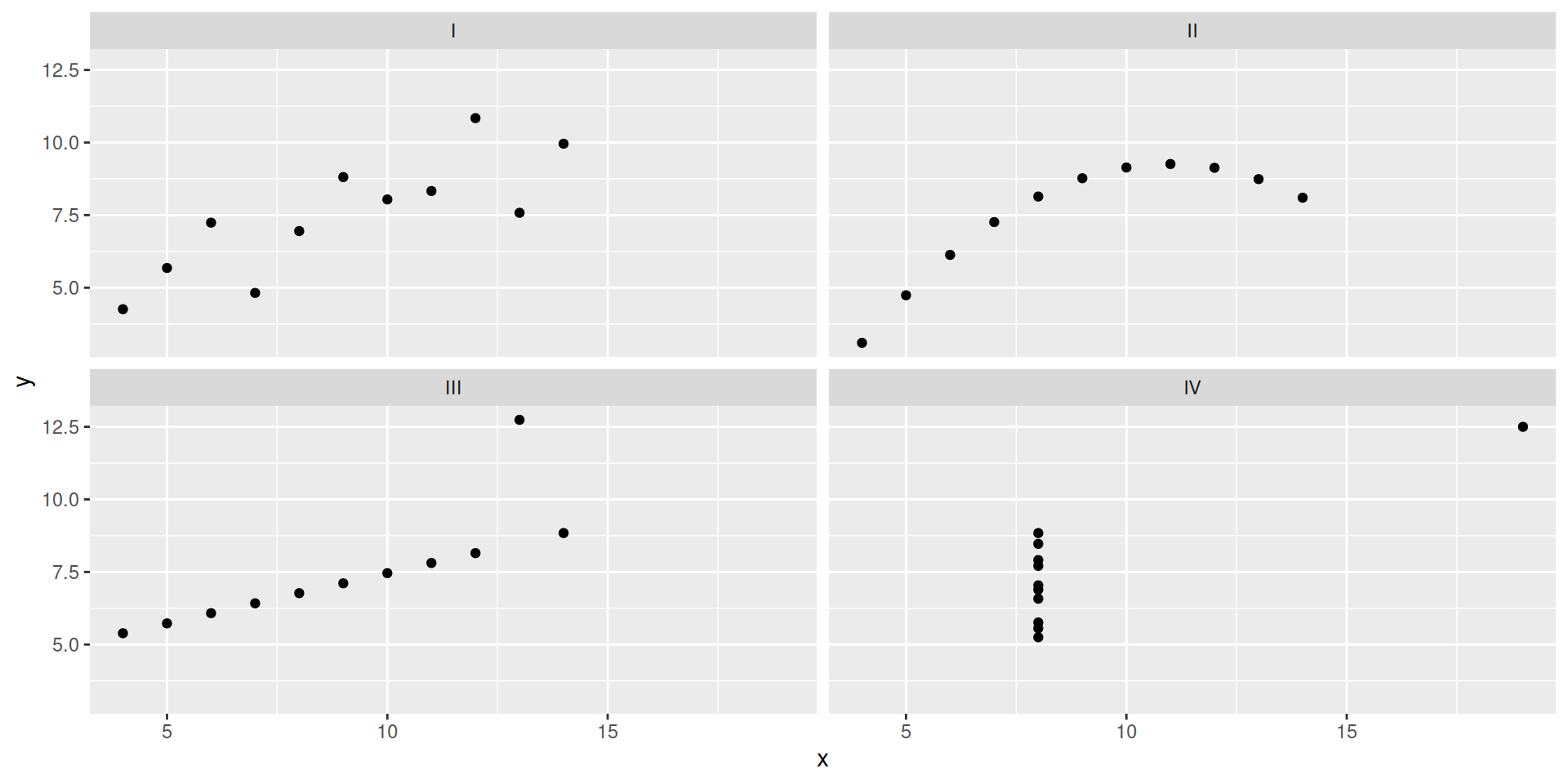
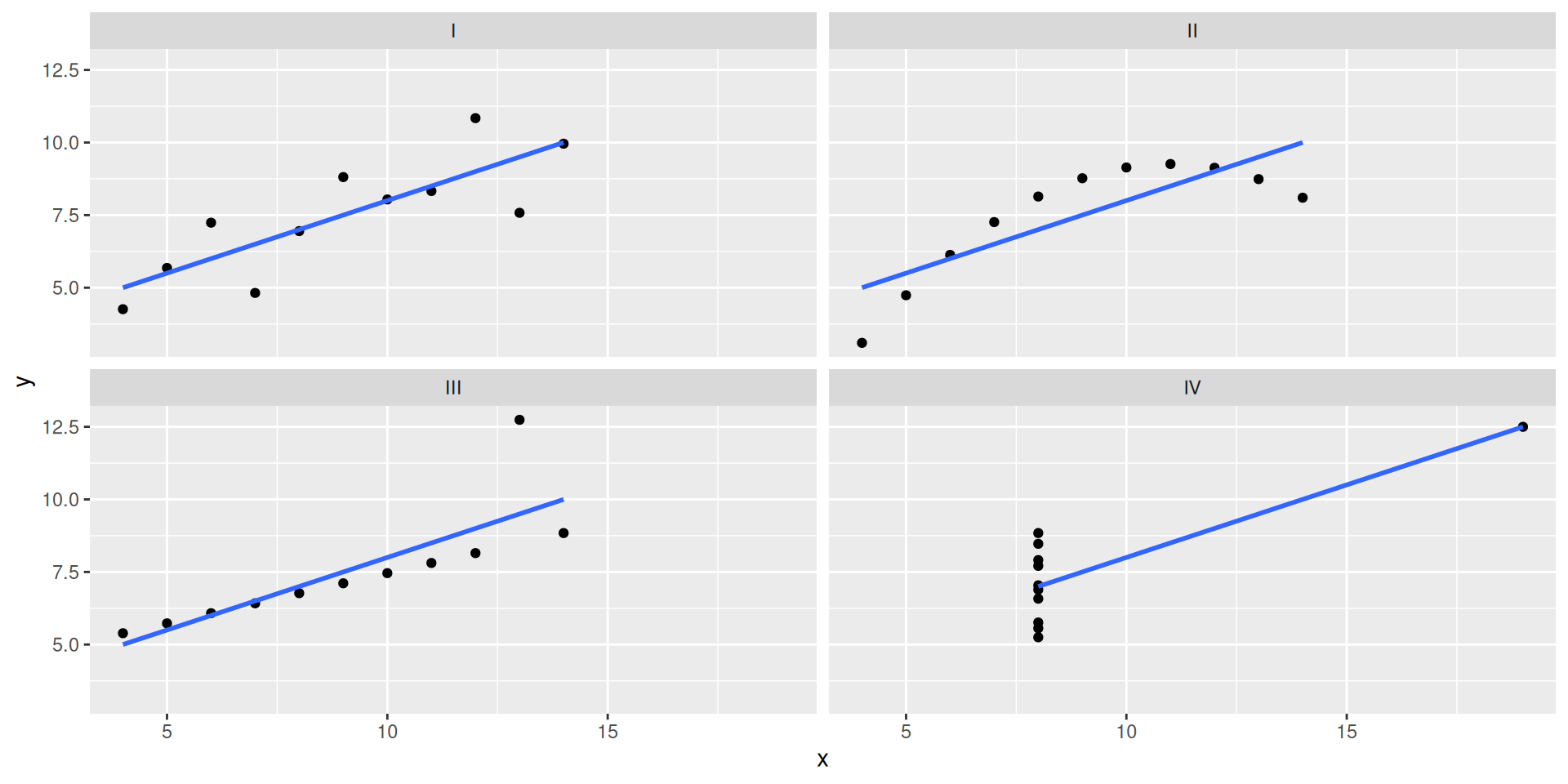
What is a line?

But on a plot…

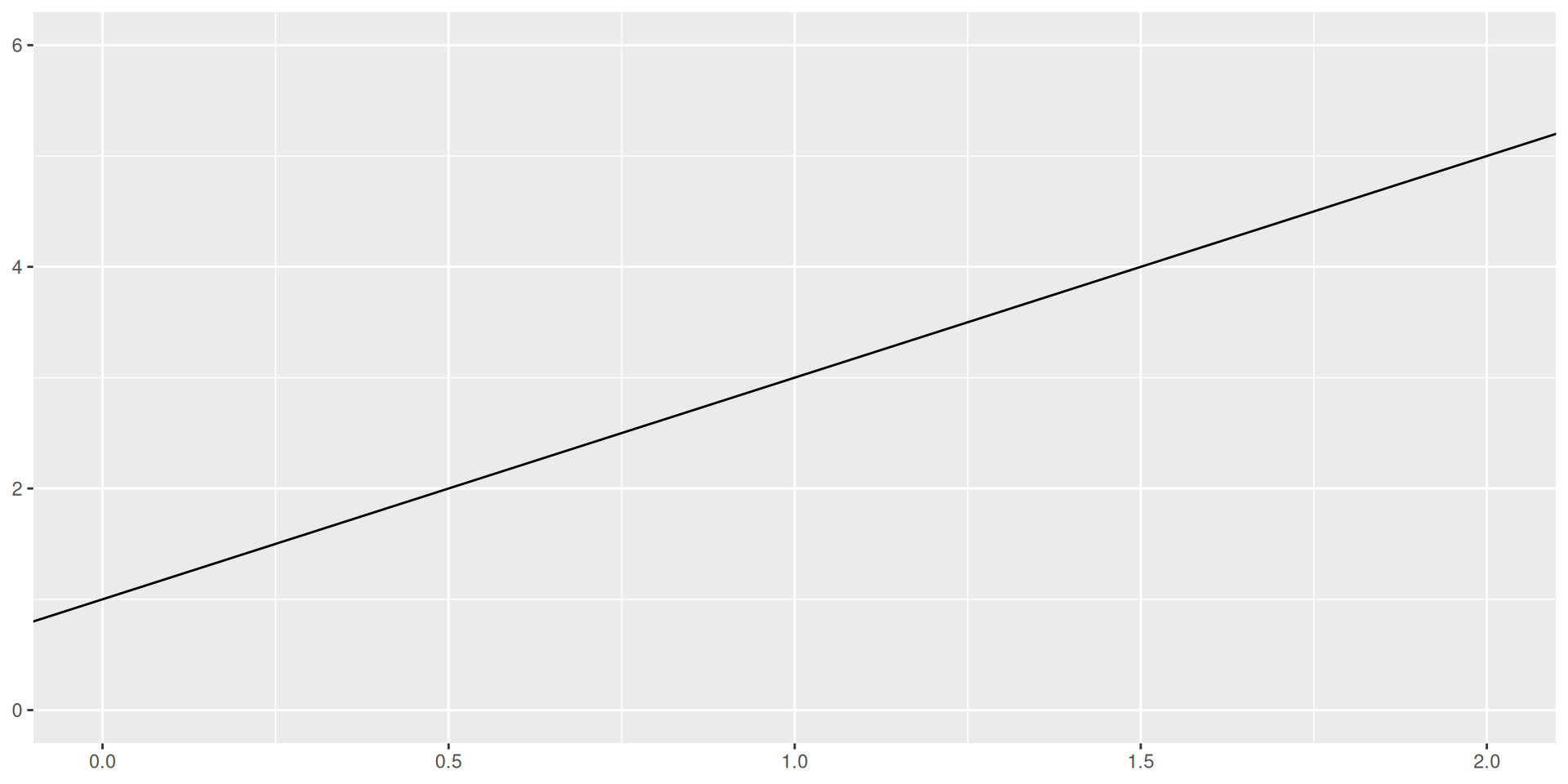
But in math terms… back to Algebra I

\[ \begin{aligned} y &= mx + b \\ \text{Output}&=\text{Slope}\times \text{Input} + \text{Intercept} \end{aligned} \]

Modeling vocabulary

• Predictor(s) (explanatory variable(s), often denoted with a subscripted “x”)
• Outcome (response variable, often denoted with “y”)
• Regression line
  • Slope (in statistics, we commonly represent slope “parameters” with a subscripted \(\beta\))
  • Intercept (in statistics, the intercept parameter is typically denoted with \(\beta_0\) )
• Correlation (more shortly)

Predictor (explanatory variable)

mpg	wt
21	2.62
21	2.875
22.8	2.32
21.4	3.215
18.7	3.44
18.1	3.46
...	...

Outcome (response variable)

mpg	wt
21	2.62
21	2.875
22.8	2.32
21.4	3.215
18.7	3.44
18.1	3.46
...	...

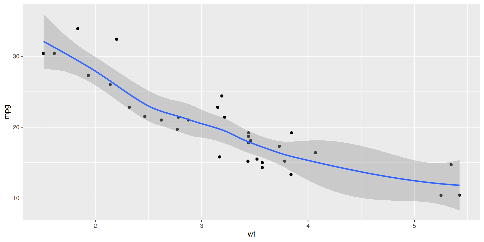
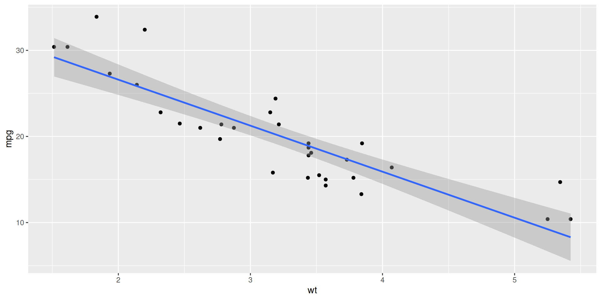
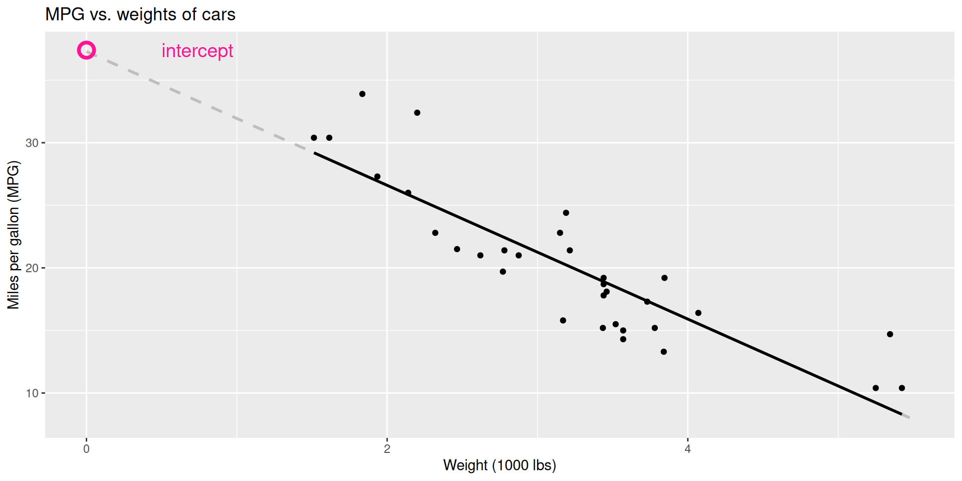
Regression line

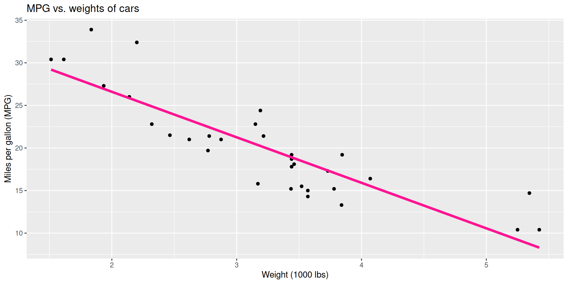
Regression line: slope

Regression line: intercept

Correlation

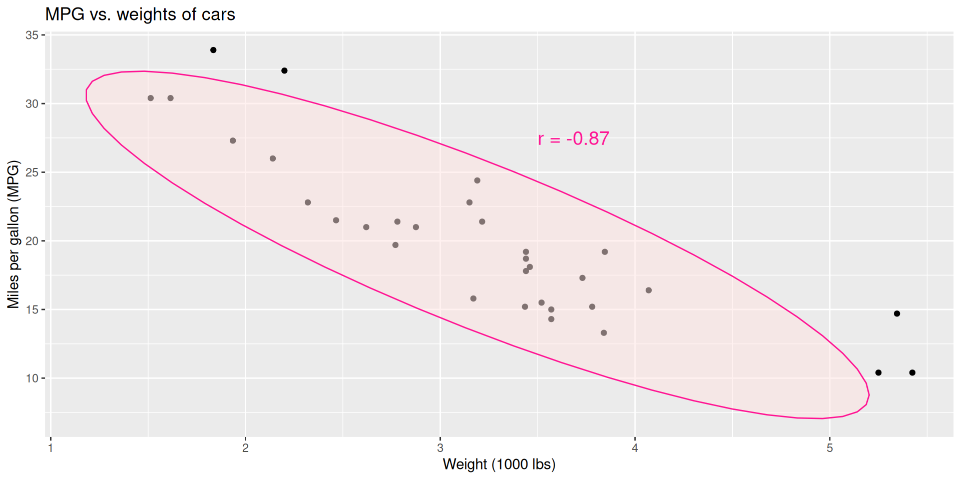
Correlation

• Measures the strength and direction of the linear association between two numerical variables;
• Tells you how tightly the points cluster around a straight line;
• Ranges between -1 and 1, inclusive;
• Same sign as the slope.

New command: cor

df

# A tibble: 140 × 4
       x series     y r    
   <int> <chr>  <dbl> <fct>
 1     1 y1      0.75 r = 1
 2     2 y1      1.5  r = 1
 3     3 y1      2.25 r = 1
 4     4 y1      3    r = 1
 5     5 y1      3.75 r = 1
 6     6 y1      4.5  r = 1
 7     7 y1      5.25 r = 1
 8     8 y1      6    r = 1
 9     9 y1      6.75 r = 1
10    10 y1      7.5  r = 1
# ℹ 130 more rows

df |>
  summarize(
    r = cor(x, y)
  )

# A tibble: 1 × 1
       r
   <dbl>
1 0.0405

Practice!

https://www.rossmanchance.com/applets/2021/guesscorrelation/GuessCorrelation.html

(Just the sort of pain in the ass visual intuition crap that I’m liable to put on an exam…)

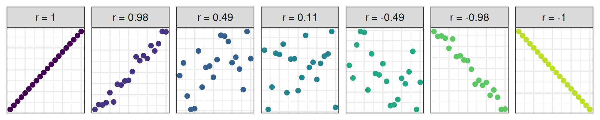
Why correlation, and not slope, as a measure of strength?

Visualizing the model

ggplot(mtcars, aes(x = wt, y = mpg)) +
  geom_point()

Visualizing the model

ggplot(mtcars, aes(x = wt, y = mpg)) +
  geom_point() + 
  geom_smooth()

`geom_smooth()` using method = 'loess' and formula = 'y ~ x'

Visualizing the model

ggplot(mtcars, aes(x = wt, y = mpg)) +
  geom_point() + 
  geom_smooth(method = "loess")

`geom_smooth()` using formula = 'y ~ x'

Visualizing the model

ggplot(mtcars, aes(x = wt, y = mpg)) +
  geom_point() + 
  geom_smooth(method = "lm")

`geom_smooth()` using formula = 'y ~ x'

Visualizing the model

ggplot(mtcars, aes(x = wt, y = mpg)) +
  geom_point() + 
  geom_smooth(method = "lm", se = FALSE)

`geom_smooth()` using formula = 'y ~ x'

Don’t forget: Always Be Visualizing!

Anscombe’s Quartet

Dataset I

    x     y
1  10  8.04
2   8  6.95
3  13  7.58
4   9  8.81
5  11  8.33
6  14  9.96
7   6  7.24
8   4  4.26
9  12 10.84
10  7  4.82
11  5  5.68

Dataset II

    x    y
1  10 9.14
2   8 8.14
3  13 8.74
4   9 8.77
5  11 9.26
6  14 8.10
7   6 6.13
8   4 3.10
9  12 9.13
10  7 7.26
11  5 4.74

Dataset III

    x     y
1  10  7.46
2   8  6.77
3  13 12.74
4   9  7.11
5  11  7.81
6  14  8.84
7   6  6.08
8   4  5.39
9  12  8.15
10  7  6.42
11  5  5.73

Dataset IV

    x     y
1   8  6.58
2   8  5.76
3   8  7.71
4   8  8.84
5   8  8.47
6   8  7.04
7   8  5.25
8  19 12.50
9   8  5.56
10  8  7.91
11  8  6.89

Very different

ggplot(anscombe_tidy, aes(x, y)) +
  geom_point() +
  facet_wrap(~ set) 

But it’s the same line…

ggplot(anscombe_tidy, aes(x, y)) +
  geom_point() +
  facet_wrap(~ set) +
  geom_smooth(method = "lm", se = FALSE)

`geom_smooth()` using formula = 'y ~ x'

…and the same summary statistics.

anscombe_tidy |>
  group_by(set) |>
  summarize(
    xbar = mean(x),
    ybar = mean(y),
    sx = sd(x),
    sy = sd(y),
    r = cor(x, y)
  )

# A tibble: 4 × 6
  set    xbar  ybar    sx    sy     r
  <chr> <dbl> <dbl> <dbl> <dbl> <dbl>
1 I         9  7.50  3.32  2.03 0.816
2 II        9  7.50  3.32  2.03 0.816
3 III       9  7.5   3.32  2.03 0.816
4 IV        9  7.50  3.32  2.03 0.817

AE-12

ae-12-modeling-fish

• Go to your ae project in RStudio.

• If you haven’t yet done so, make sure all of your changes up to this point are committed and pushed, i.e., there’s nothing left in your Git pane.

• If you haven’t yet done so, click Pull to get today’s application exercise file: ae-12-modeling-fish.qmd.

• Work through the application exercise in class, and render, commit, and push your edits.

New commands introduced today

In base R:

• cor: compute correlation between two numerical variables;

In ggplot2:

• geom_smooth(method = "lm"): add linear model line of best fit to scatterplot;

In the new package tidymodels:

• linear_reg and fit: estimate linear model;
• tidy: cute lil’ summary table of model output;
• predict: use estimated model to predict.