Multiple Linear Regression 1
Lecture 14
June 5, 2026
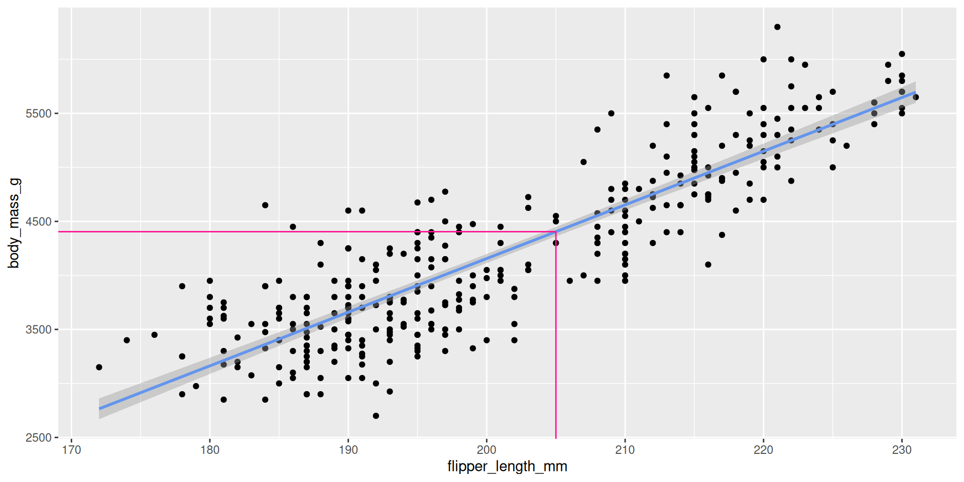
Line of best fit!
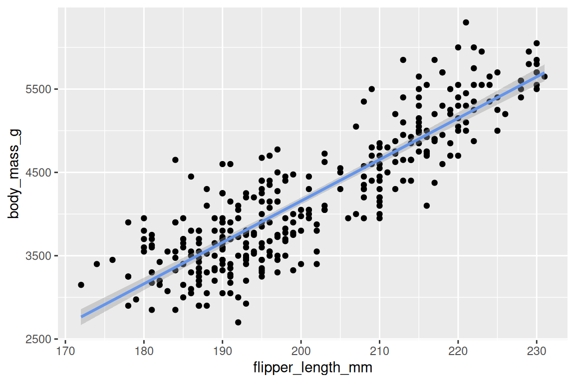
Prediction
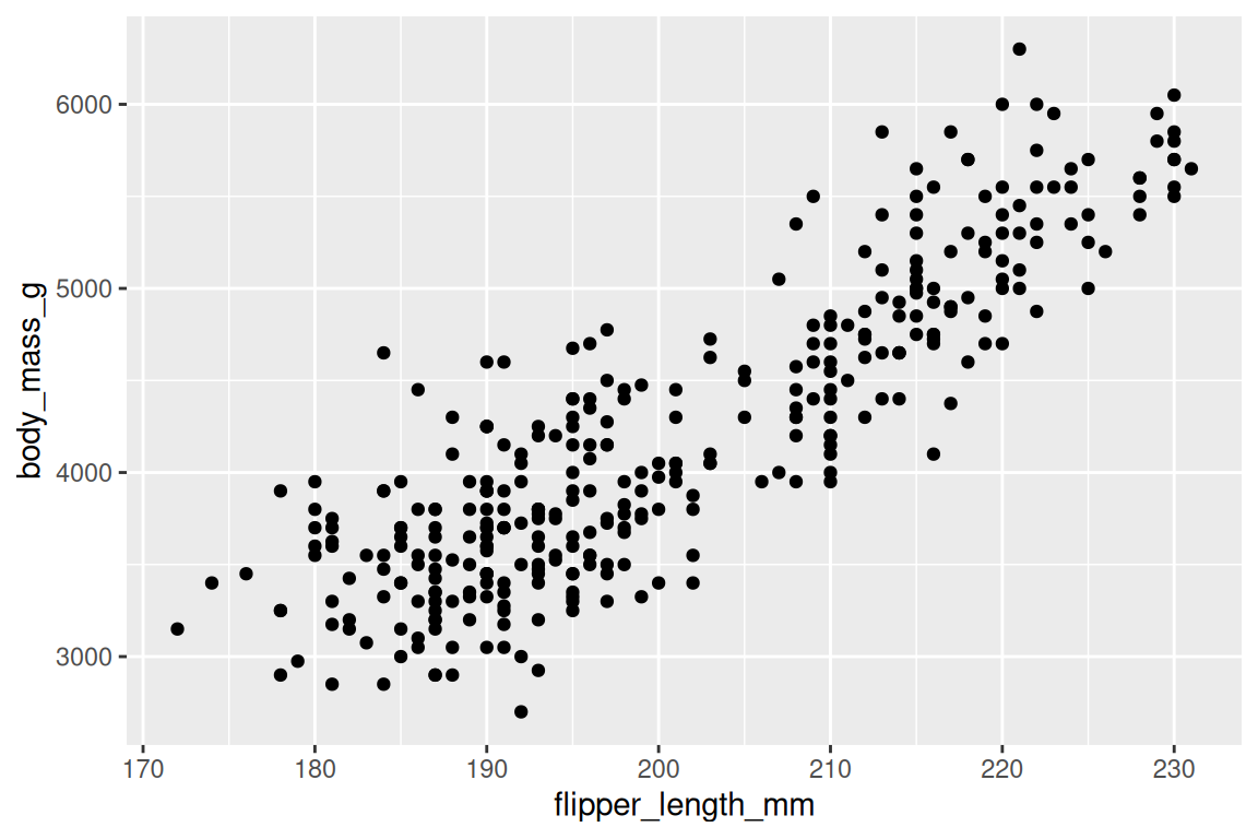
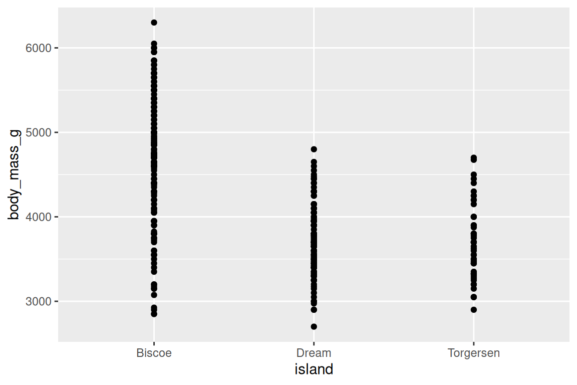
Scatterplot: possible, but not so good
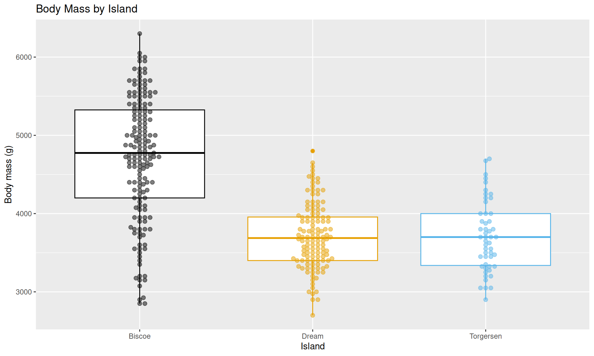
Visualize the relationship between body weight and island of penguins. Also calculate the average body weight per island.
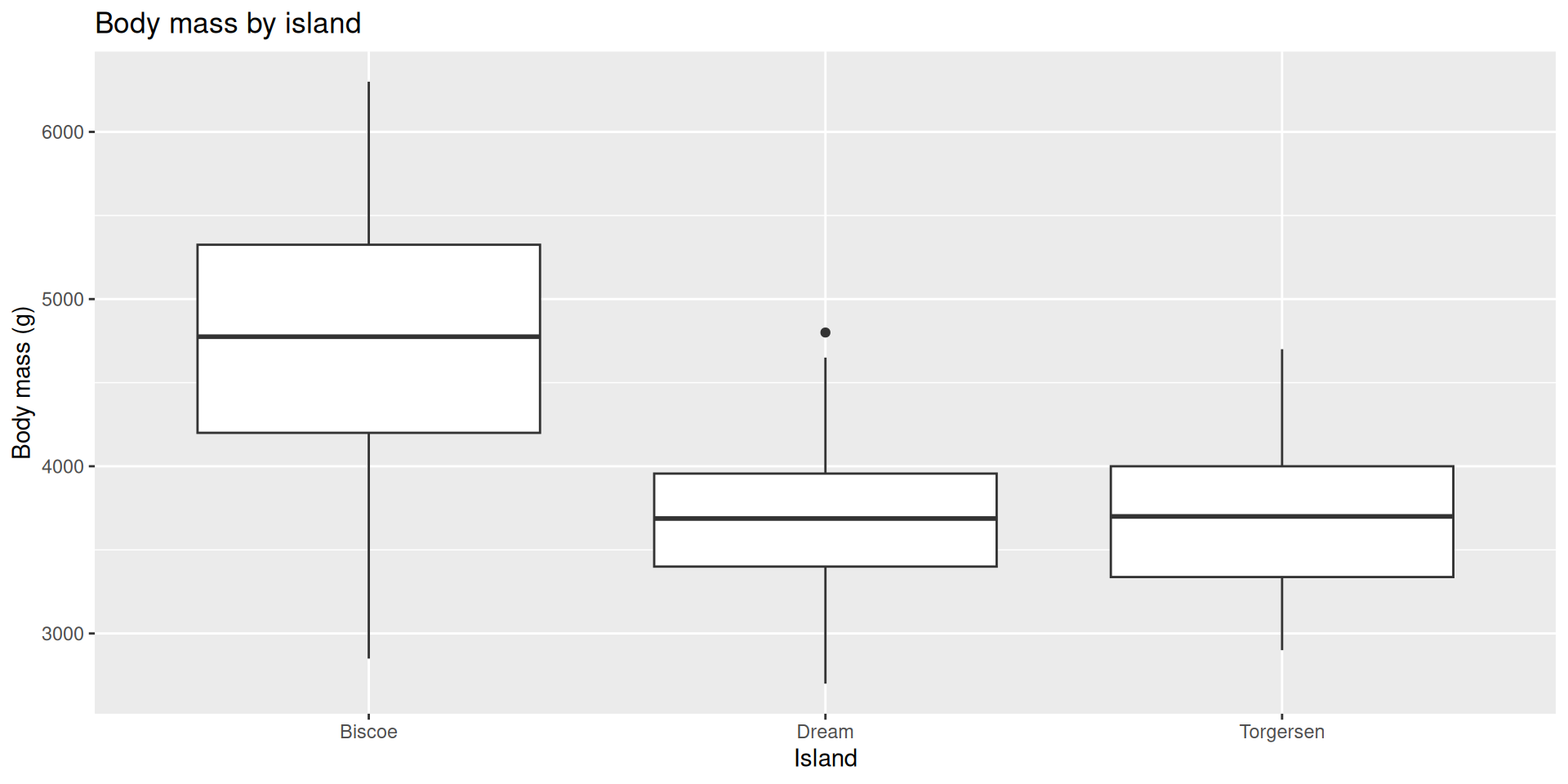
Boxplot
Visualize the relationship between body weight and island of penguins. Also, calculate the average body weight per island.
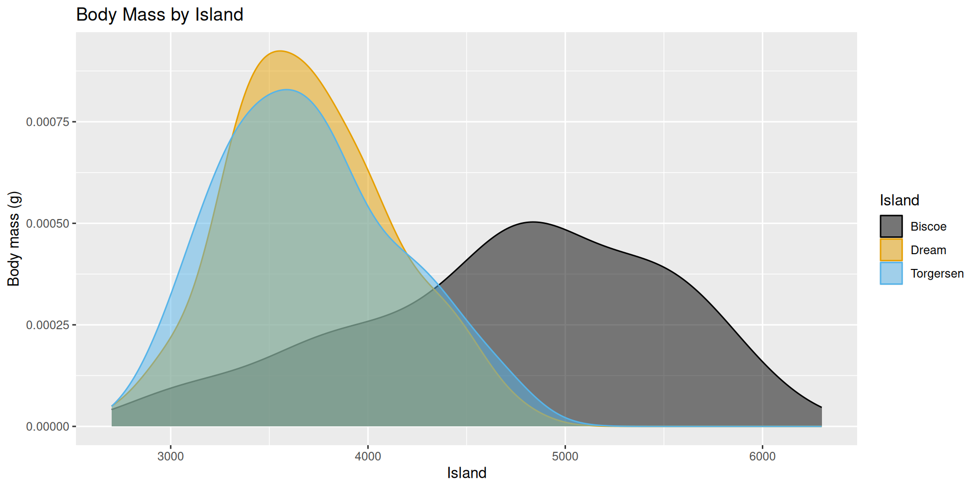
Density plot
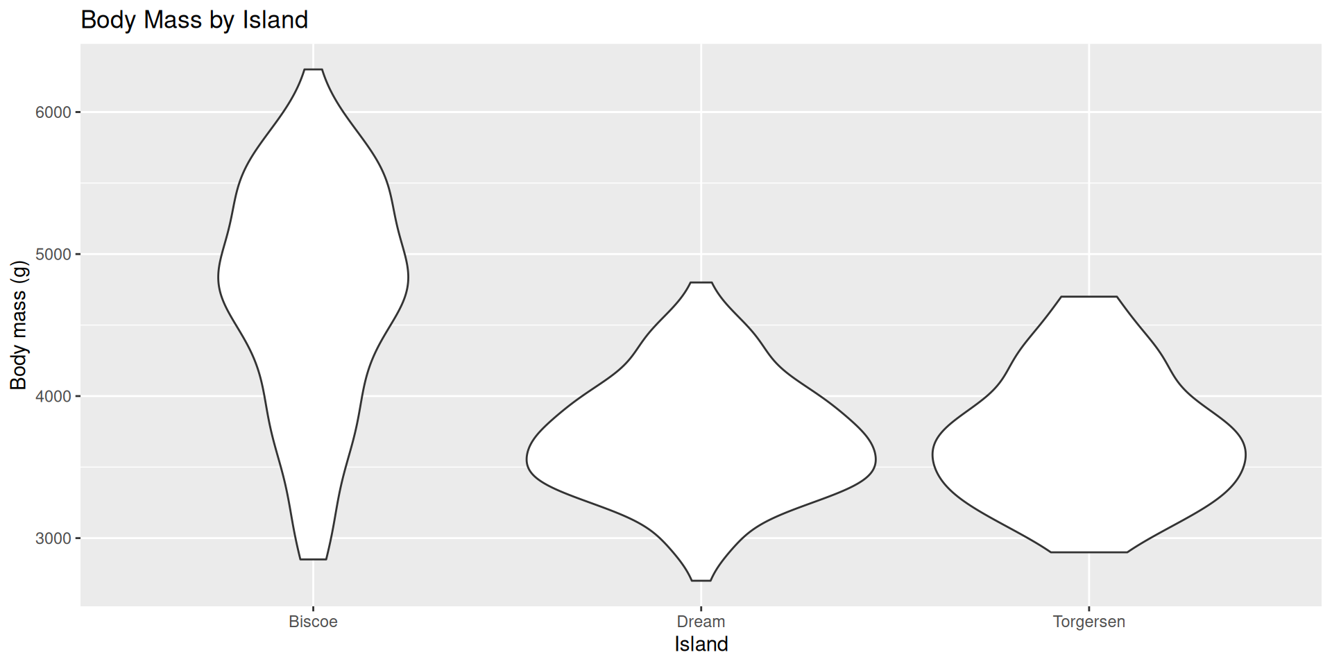
Violin plot
Multiple geoms
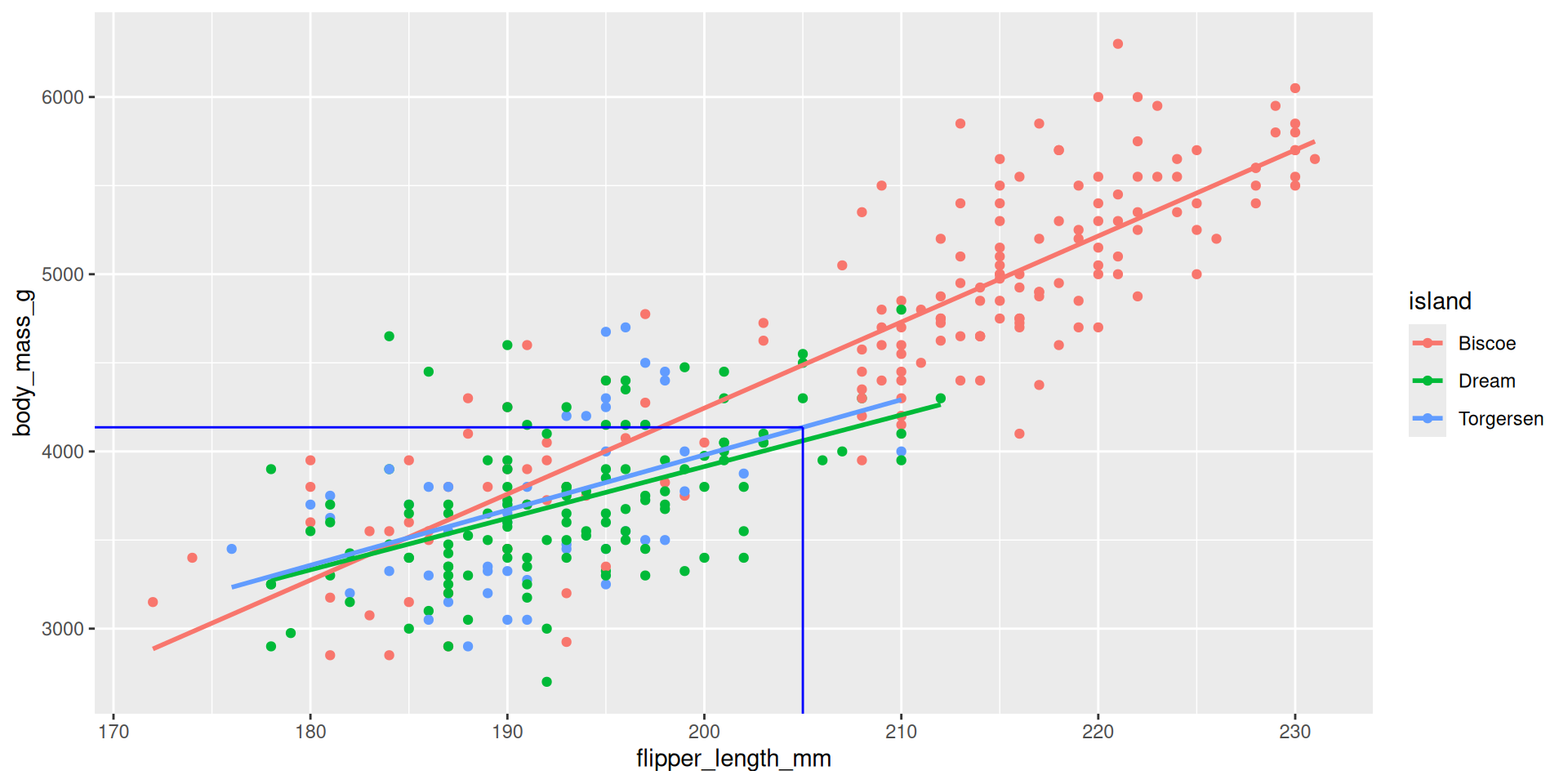
Three variables on one 2D plot
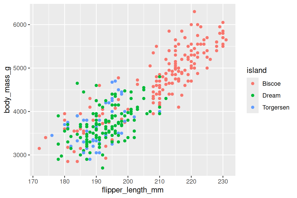
How do we predict using more than one predictor?
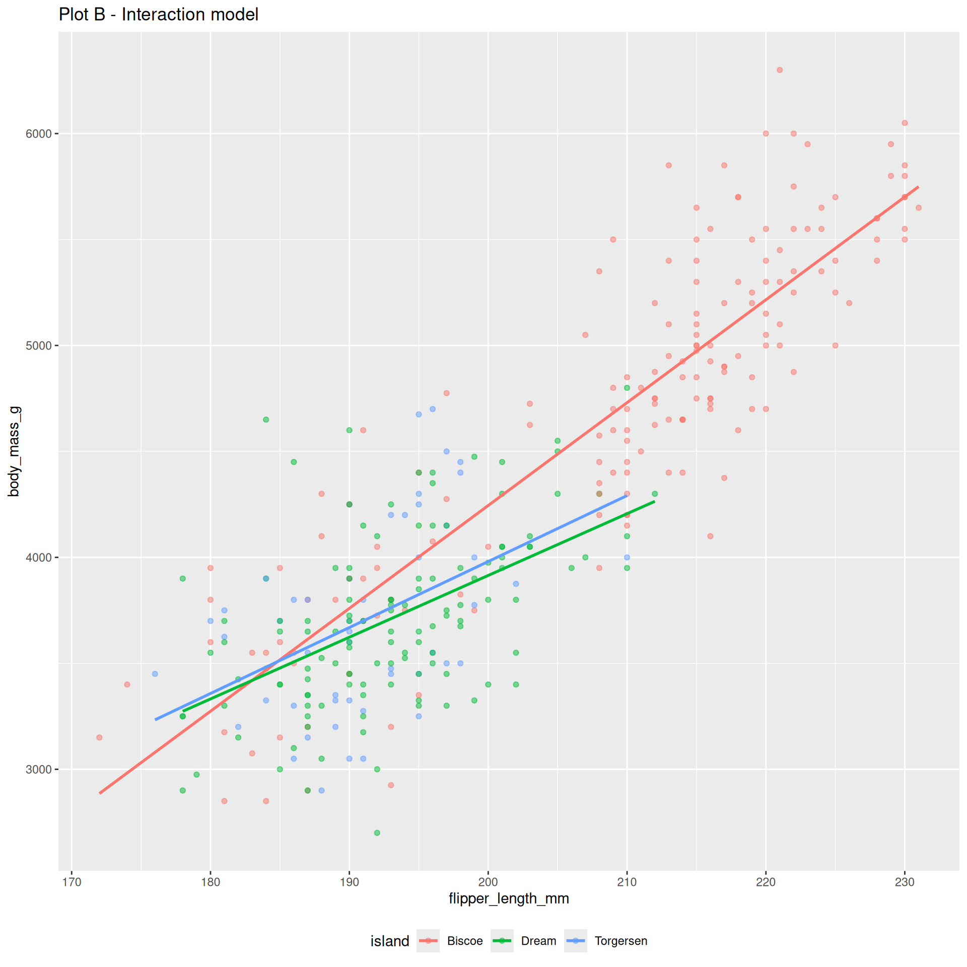
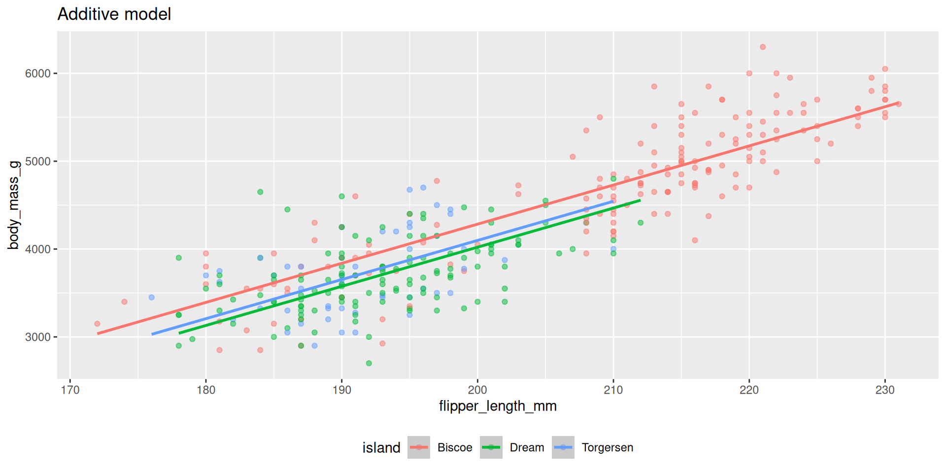
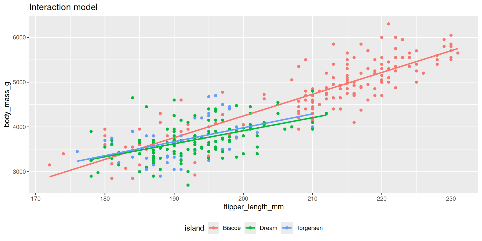
Both of these models use flipper_length_mm and island to predict body_mass_g:
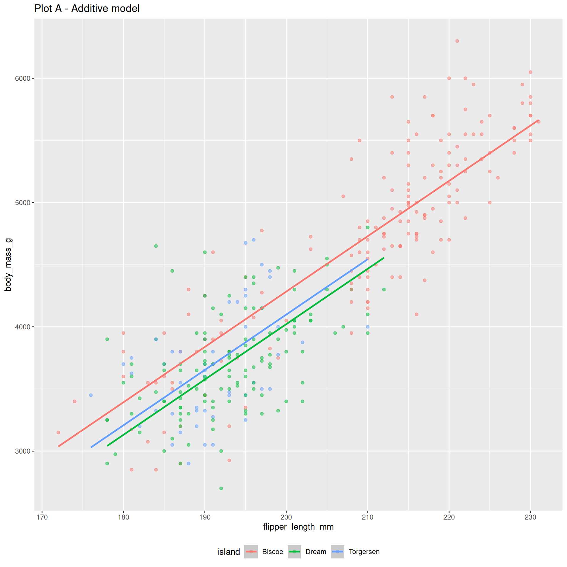
The additive model: parallel lines, one for each island
The interaction model: different lines for each island
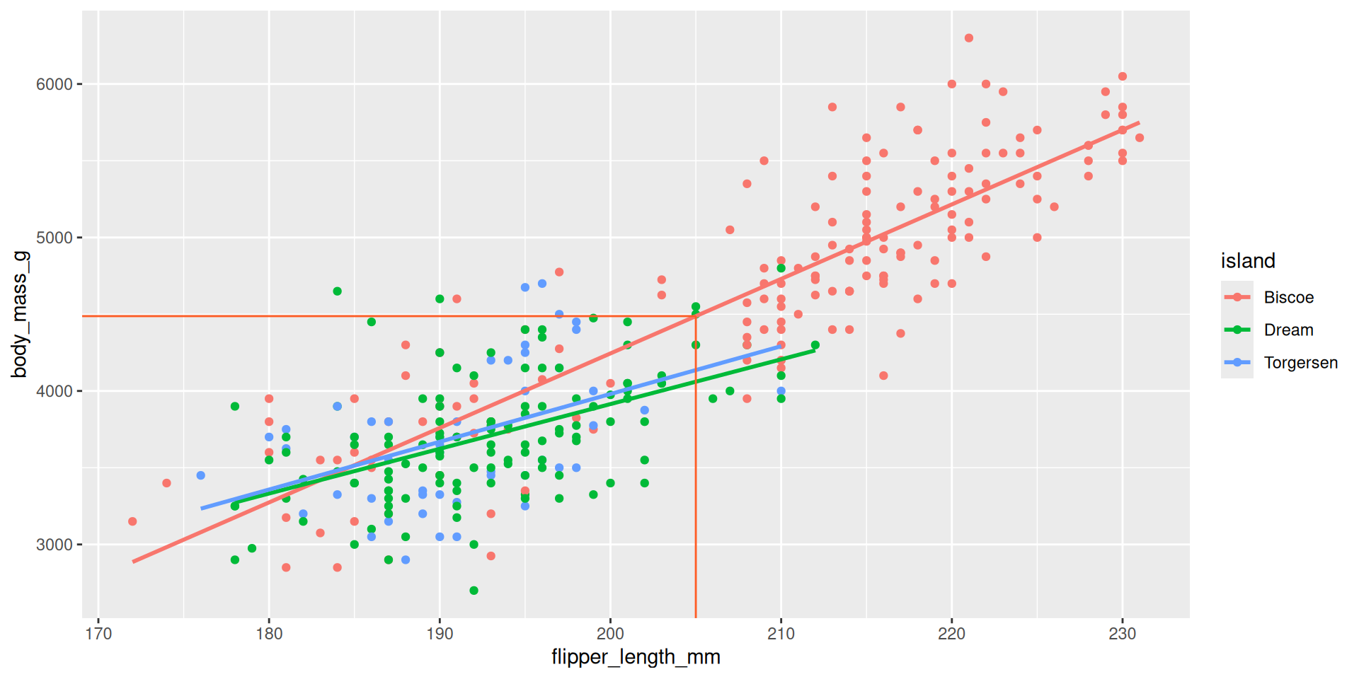
Prediction on Biscoe island
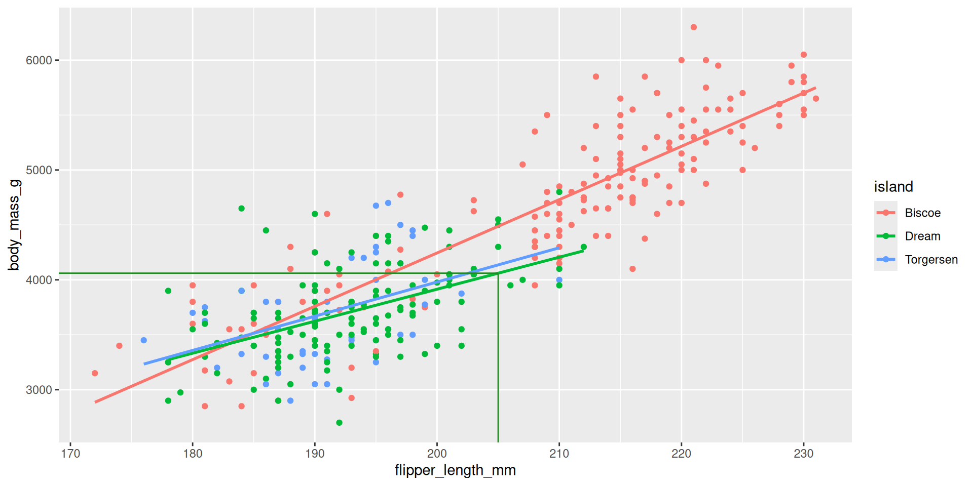
Prediction on Dream island
Prediction on Torgersen island
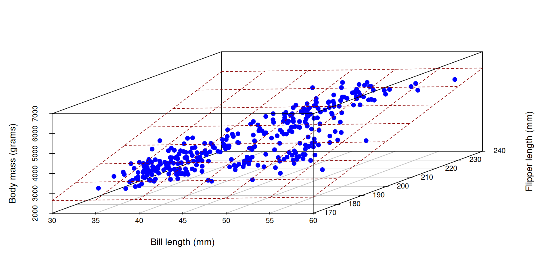
Picture? It’s not pretty…
2 predictors + 1 response = 3 dimensions. Ick!
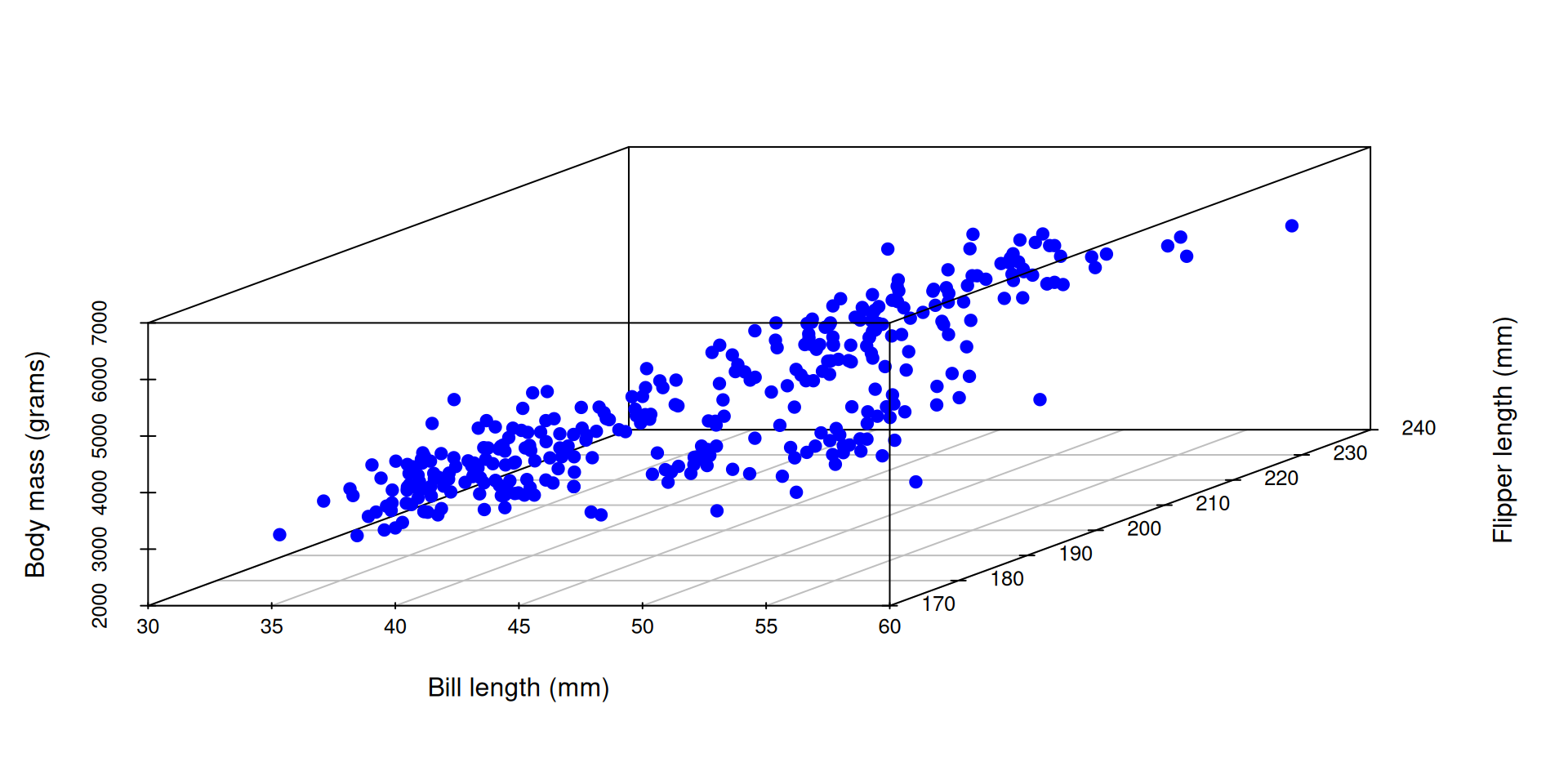
Picture? It’s not pretty…
Instead of a line of best fit, it’s a plane of best fit. Double ick!