# A tibble: 2 × 2
  term        estimate
  <chr>          <dbl>
1 (Intercept)    2.94
2 log_inc 0.657Lecture 20
# A tibble: 2 × 2
term estimate
<chr> <dbl>
1 (Intercept) 2.94
2 log_inc 0.657
# A tibble: 2 × 2
  term        estimate
  <chr>          <dbl>
1 (Intercept)    5.29
2 log_inc        0.486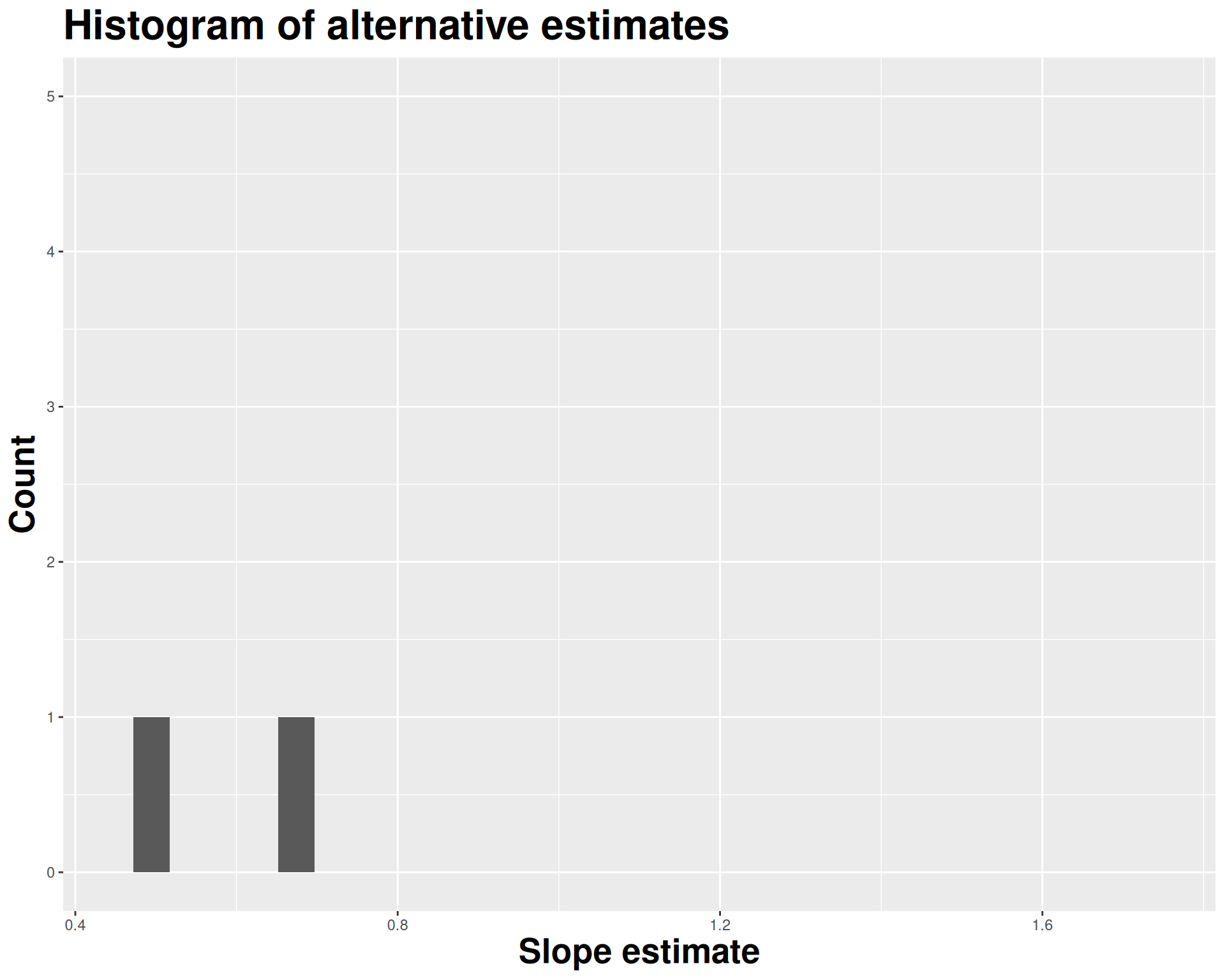
# A tibble: 2 × 2
  term        estimate
  <chr>          <dbl>
1 (Intercept)    1.62
2 log_inc        0.805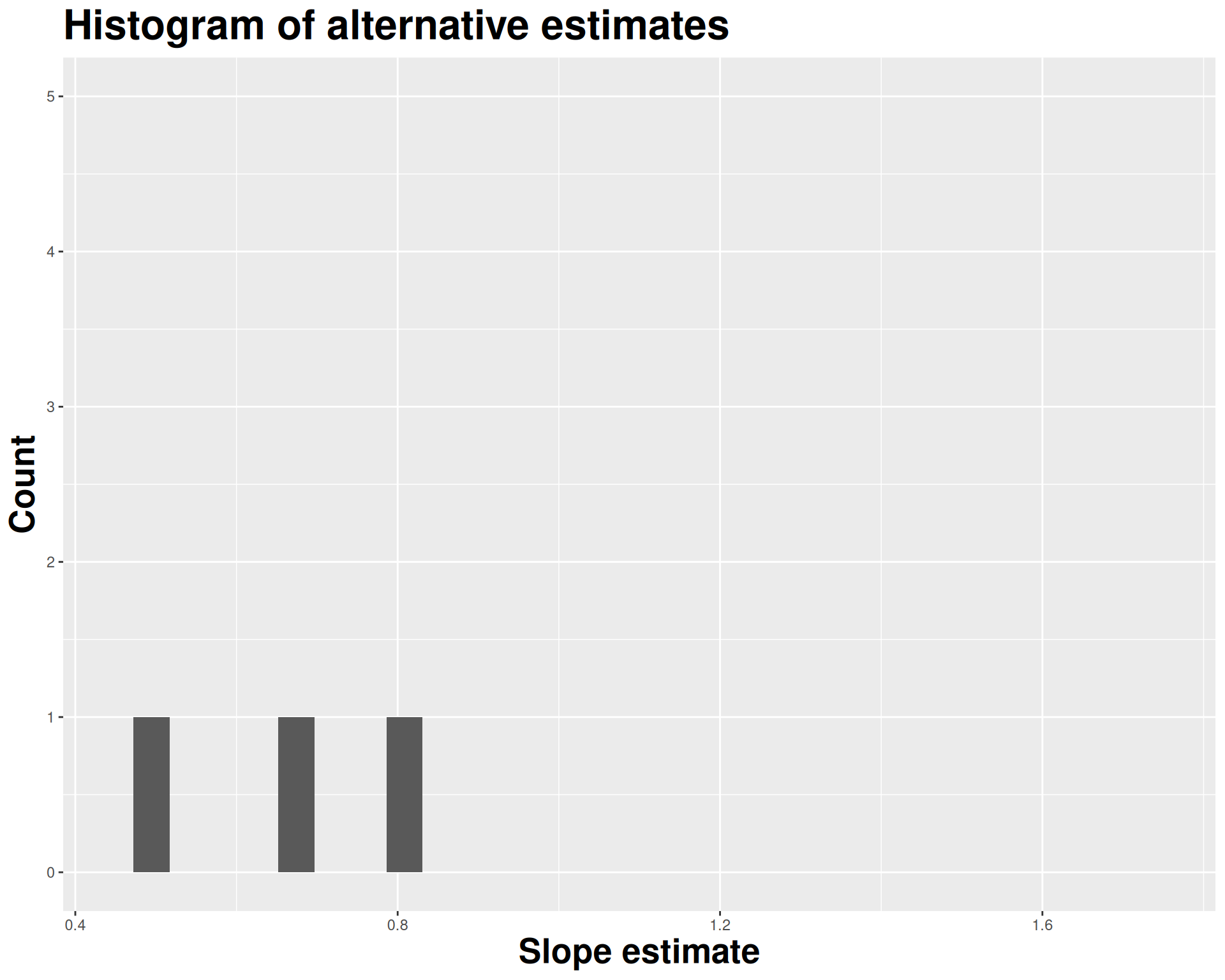
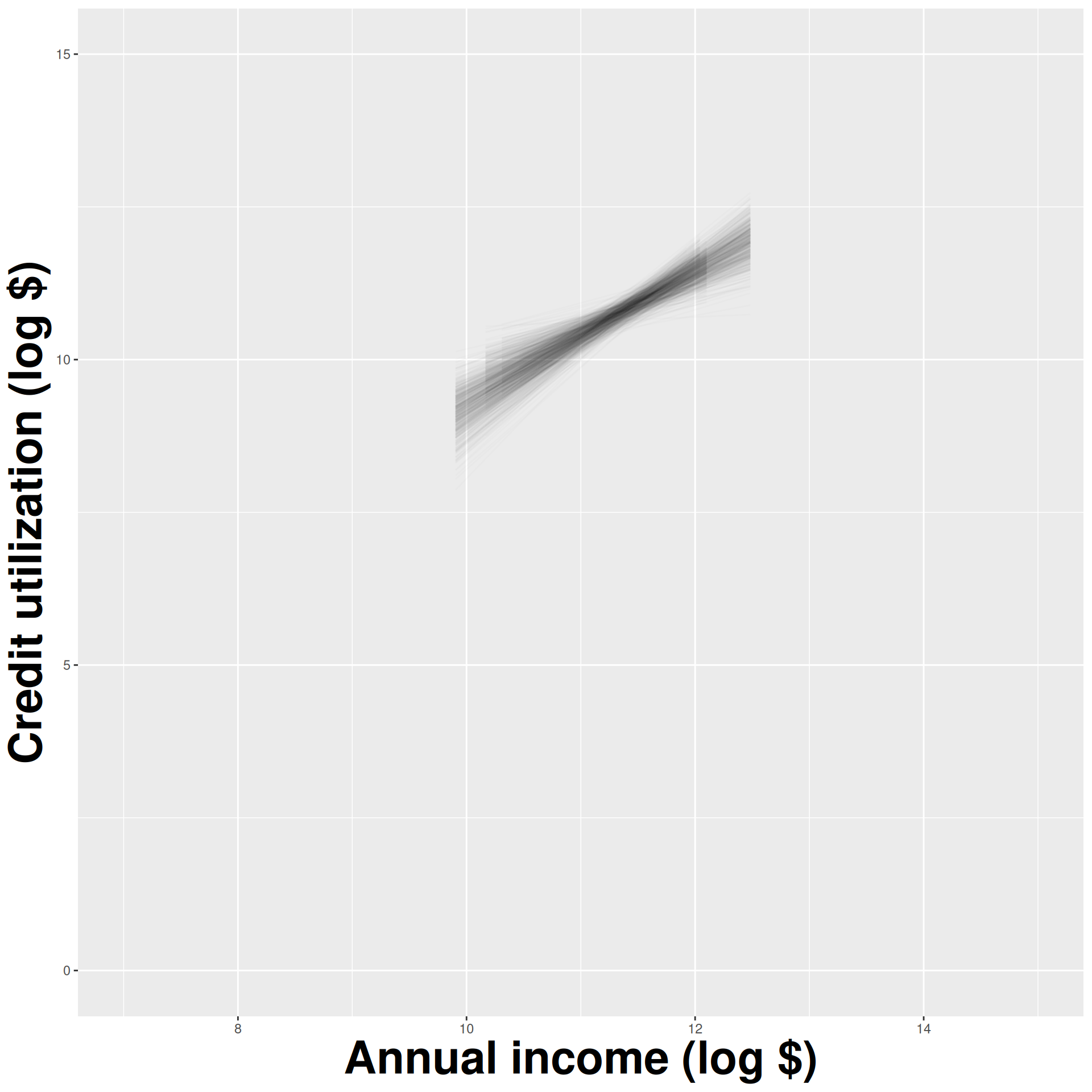
How sensitive are the estimates to the data they are based on?
- Very? Then uncertainty is high, results are unreliable;
- Not very? Uncertainty is low, results are more reliable.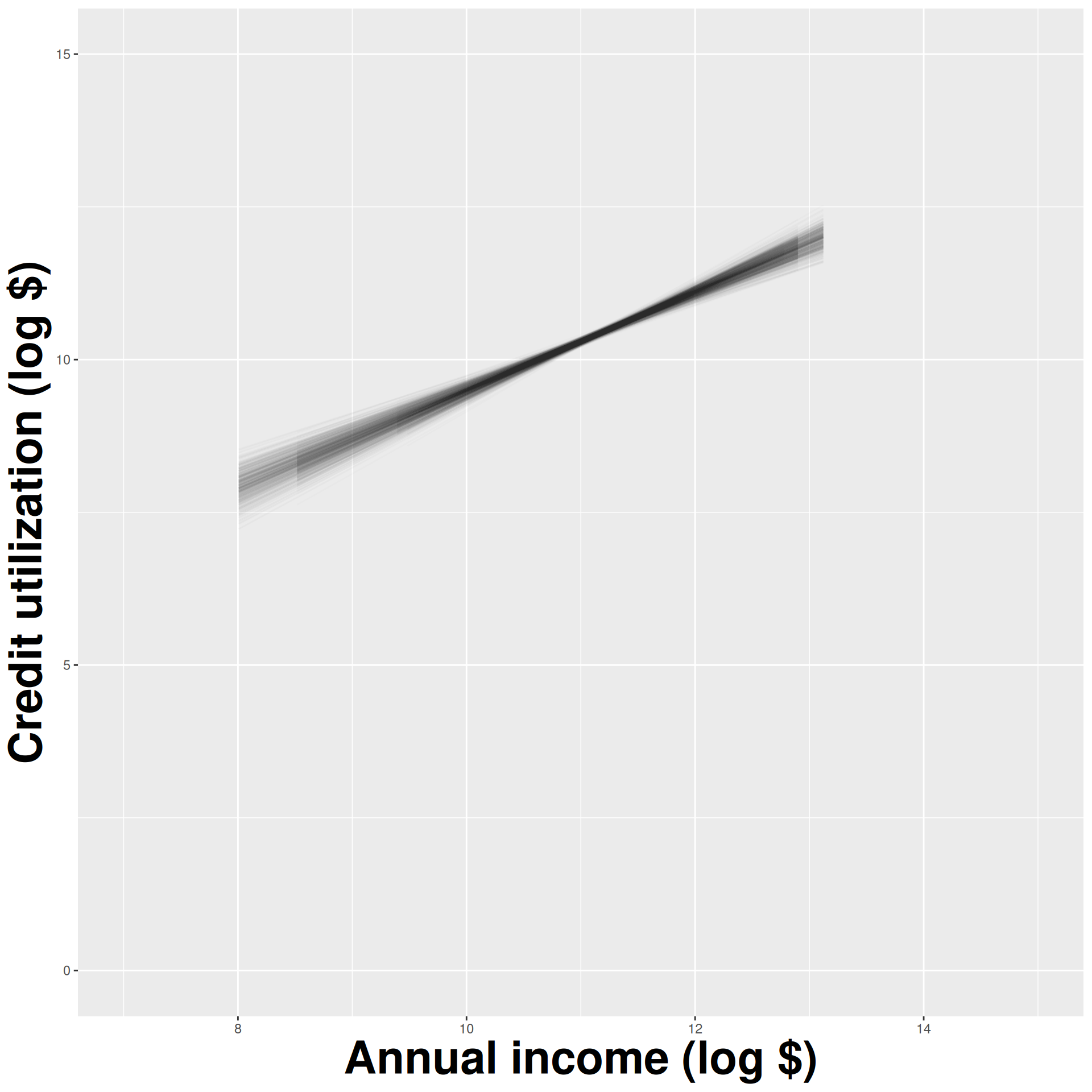
Data collection is costly, so we have to do our best with what we already have;
We approximate this idea of “alternative, hypothetical datasets I could have observed” by resampling our data with replacement;
We construct a new dataset of the same size by randomly picking rows out of the original one:
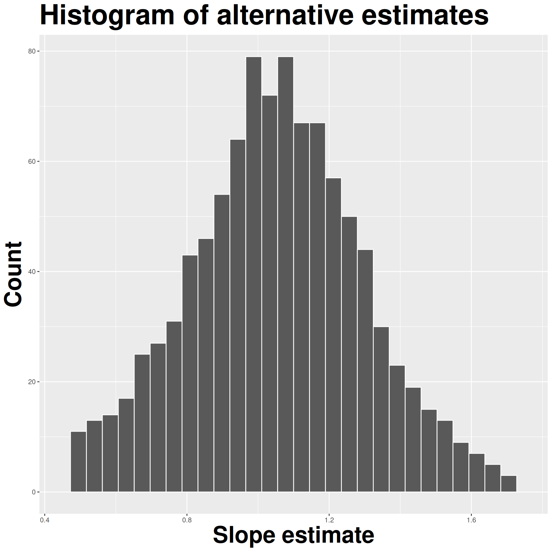
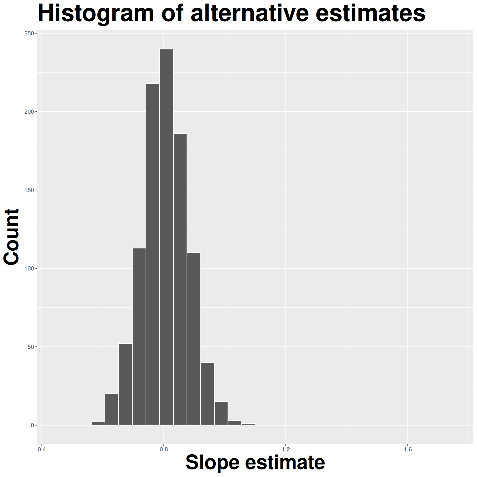
Repeat this processes hundred or thousands of times, and observe how the estimates vary as you refit the model on alternative datasets.
This gives you a sense of the sampling variability of your estimates.
Original data
# A tibble: 6 × 3
     id       x       y
  <int>   <dbl>   <dbl>
1     1  0.432   1.53
2     2 -2.01    1.80
3     3 -0.0467  1.43
4     4 -1.05    0.0518
5     5  0.327   0.820
6     6 -0.679  -0.961
Original estimates:
# A tibble: 2 × 2
  term        estimate
  <chr>          <dbl>
1 (Intercept)   0.801
2 x             0.0450
Sample with replacement:
# A tibble: 6 × 3
     id      x      y
  <int>  <dbl>  <dbl>
1     5  0.327  0.820
2     6 -0.679 -0.961
3     6 -0.679 -0.961
4     1  0.432  1.53
5     6 -0.679 -0.961
6     1  0.432  1.53
Different data \(\rightarrow\) new estimates:
# A tibble: 2 × 2
  term        estimate
  <chr>          <dbl>
1 (Intercept)    0.462
2 x 2.11 Original data
# A tibble: 6 × 3
     id       x       y
  <int>   <dbl>   <dbl>
1     1  0.432   1.53
2     2 -2.01    1.80
3     3 -0.0467  1.43
4     4 -1.05    0.0518
5     5  0.327   0.820
6     6 -0.679  -0.961
Original estimates:
# A tibble: 2 × 2
  term        estimate
  <chr>          <dbl>
1 (Intercept)   0.801
2 x             0.0450
Sample with replacement:
# A tibble: 6 × 3
     id       x      y
  <int>   <dbl>  <dbl>
1     2 -2.01    1.80
2     5  0.327   0.820
3     1  0.432   1.53
4     6 -0.679  -0.961
5     3 -0.0467  1.43
6     2 -2.01    1.80
Different data \(\rightarrow\) new estimates:
# A tibble: 2 × 2
  term        estimate
  <chr>          <dbl>
1 (Intercept)    0.913
2 x -0.236Original data
# A tibble: 6 × 3
     id       x       y
  <int>   <dbl>   <dbl>
1     1  0.432   1.53
2     2 -2.01    1.80
3     3 -0.0467  1.43
4     4 -1.05    0.0518
5     5  0.327   0.820
6     6 -0.679  -0.961
Original estimates:
# A tibble: 2 × 2
  term        estimate
  <chr>          <dbl>
1 (Intercept)   0.801
2 x             0.0450
Sample with replacement:
# A tibble: 6 × 3
     id      x      y
  <int>  <dbl>  <dbl>
1     6 -0.679 -0.961
2     1  0.432  1.53
3     5  0.327  0.820
4     6 -0.679 -0.961
5     6 -0.679 -0.961
6     5  0.327  0.820
Different data \(\rightarrow\) new estimates:
# A tibble: 2 × 2
  term        estimate
  <chr>          <dbl>
1 (Intercept)    0.357
2 x 1.96 Point estimation: report your single number best guess for the unknown quantity;
Interval estimation: report a range, or interval, or values where you think the unknown quantity is likely to live;
Unfortunately, there is a trade-off. You adjust the confidence level to try to negotiate the trade-off;
Common choices: 90%, 95%, 99%.

openintro::duke_forest

Goal: Use the area (in square feet) to understand variability in the price of houses in Duke Forest.
df_fit <- linear_reg() |>
  fit(price ~ area, data = duke_forest)

tidy(df_fit) |>
kable(digits = 2) # neatly format table to 2 digits| term | estimate | std.error | statistic | p.value |
|---|---|---|---|---|
| (Intercept) | 116652.33 | 53302.46 | 2.19 | 0.03 |
| area | 159.48 | 18.17 | 8.78 | 0.00 |
A confidence interval will allow us to make a statement like “For each additional square foot, the model predicts the sale price of Duke Forest houses to be higher, on average, by $159, plus or minus X dollars.”
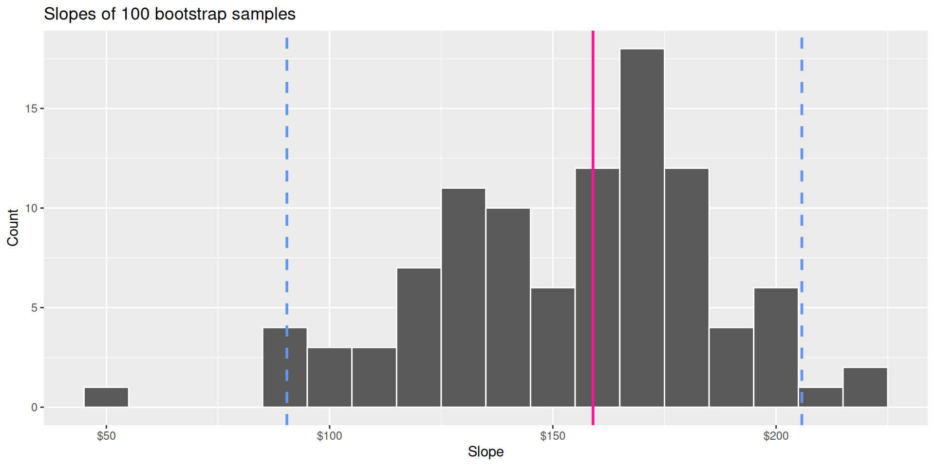
Quantiles!
90% of the bootstrap distribution is between the 5% quantile on the left and the 95% quantile on the right;
95% of the bootstrap distribution is between the 2.5% quantile on the left and the 97.5% quantile on the right;
And so on.
Calculate the observed slope:
observed_fit <- duke_forest |>
  specify(price ~ area) |>
  fit()

observed_fit
# A tibble: 2 × 2
term estimate
<chr> <dbl>
1 intercept 116652.
2 area 159.Take 100 bootstrap samples and fit models to each one:
set.seed(1120)

boot_fits <- duke_forest |>
  specify(price ~ area) |>
  generate(reps = 100, type = "bootstrap") |>
  fit()

boot_fits
# A tibble: 200 × 3
# Groups: replicate [100]
replicate term estimate
<int> <chr> <dbl>
1 1 intercept 47819.
2 1 area 191.
3 2 intercept 144645.
4 2 area 134.
5 3 intercept 114008.
6 3 area 161.
7 4 intercept 100639.
8 4 area 166.
9 5 intercept 215264.
10 5 area 125.
# ℹ 190 more rowsPercentile method: Compute the 95% CI as the middle 95% of the bootstrap distribution:
get_confidence_interval(
  boot_fits,
  point_estimate = observed_fit,
  level = 0.95,
  type = "percentile" # default method
)
# A tibble: 2 × 3
term lower_ci upper_ci
<chr> <dbl> <dbl>
1 area 92.1 223.
2 intercept -36765. 296528.If we did it manually…
How would you modify the following code to calculate a 90% confidence interval? How would you modify it for a 99% confidence interval?
## confidence level: 90%
get_confidence_interval(
  boot_fits, point_estimate = observed_fit,
  level = 0.90, type = "percentile"
)
# A tibble: 2 × 3
term lower_ci upper_ci
<chr> <dbl> <dbl>
1 area 104. 212.
2 intercept -24380. 256730.## confidence level: 99%
get_confidence_interval(
boot_fits, point_estimate = observed_fit,
level = 0.99, type = "percentile"
)# A tibble: 2 × 3
term lower_ci upper_ci
<chr> <dbl> <dbl>
1 area 56.3 226.
2 intercept -61950. 370395.Population: Complete set of observations of whatever we are studying, e.g., people, tweets, photographs, etc. (population size = \(N\))
Sample: Subset of the population, ideally random and representative (sample size = \(n\))
Sample statistic \(\ne\) population parameter, but if the sample is good, it can be a good estimate
Statistical inference: Discipline that concerns itself with the development of procedures, methods, and theorems that allow us to extract meaning and information from data that has been generated by stochastic (random) process
We report the estimate with a confidence interval, and the width of this interval depends on the variability of sample statistics from different samples from the population
Since we can’t continue sampling from the population, we bootstrap from the one sample we have to estimate sampling variability
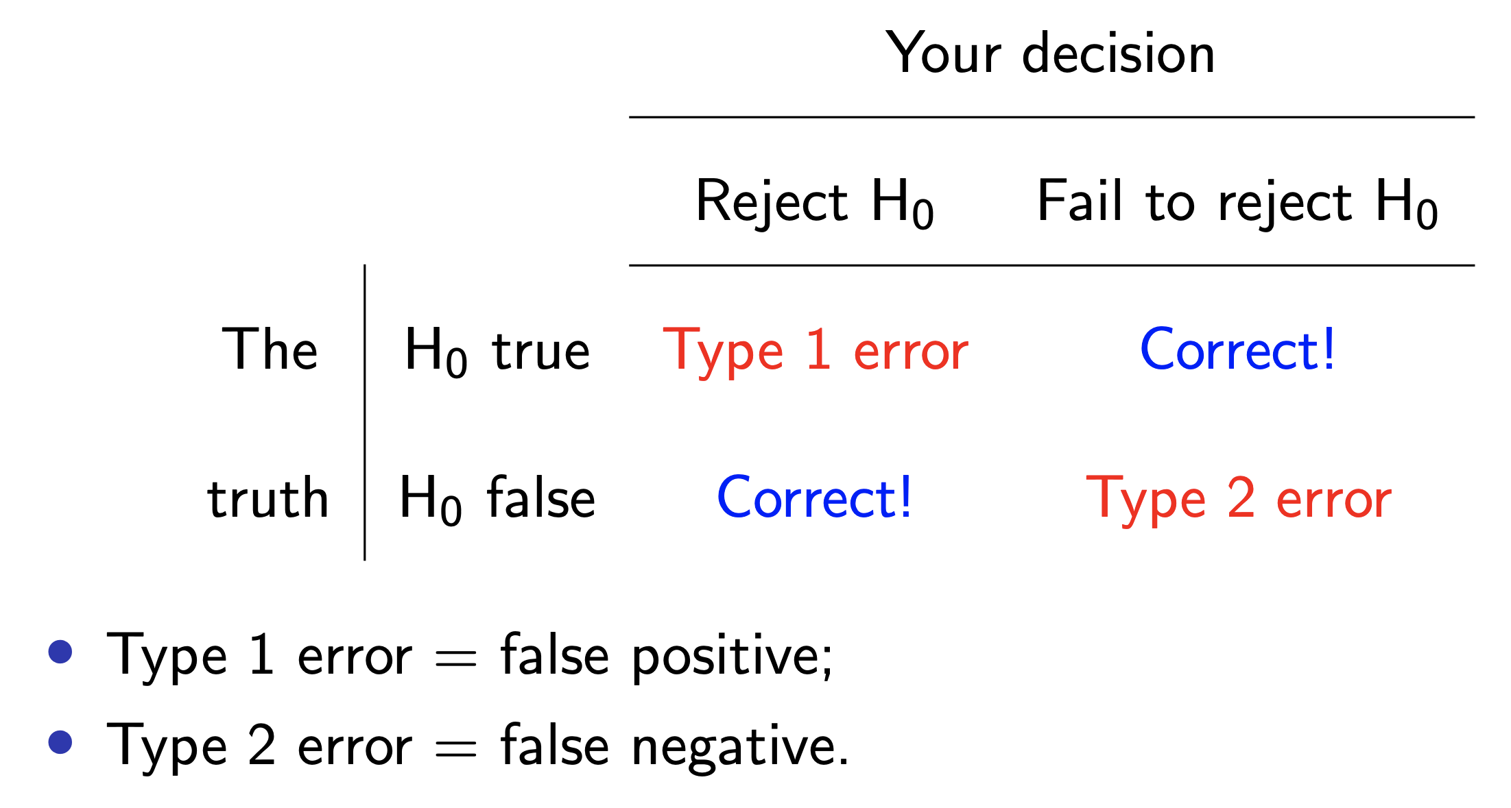
A hypothesis test is a statistical technique used to evaluate competing claims using data
Null hypothesis, \(H_0\): An assumption about the population. With respect to the slope parameter, our null hypothesis is one of “no relationship”
Alternative hypothesis, \(H_A\): A research question about the population. With respect to the slope parameter, our alternative hypothesis is that “there is some relationship”
. . .
Note: Hypotheses are always at the population level!
Null hypothesis, \(H_0\): “There is no relationship.” The slope of the model for predicting the prices of houses in Duke Forest from their areas is 0, \(\beta_1 = 0\).
Alternative hypothesis, \(H_A\): “There is some relationship”. The slope of the model for predicting the prices of houses in Duke Forest from their areas is different than 0, \(\beta_1 \ne 0\).
Assume you live in a world where null hypothesis is true: \(\beta_1 = 0\).
Ask yourself how likely you are to observe the sample statistic, or something even more extreme, in this world: \(P(b_1 \leq -159.48~or~b_1 \geq 159.48 | \beta_1 = 0)\) = ?
In words: “Given the null hypothesis is true and \(\beta_1 = 0\), what is the probability of observing \(b_1 \leq -159.48\) or \(b_1 \geq 159.48\)?”
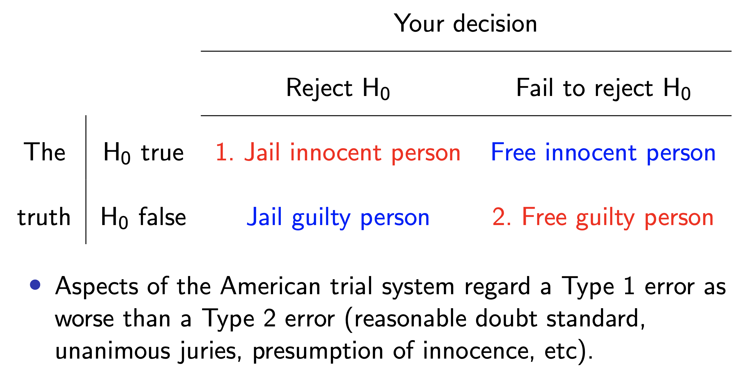
Innocent until proven guilty!
Null hypothesis, \(H_0\): Defendant is innocent
Alternative hypothesis, \(H_A\): Defendant is guilty
. . .
. . .
Null hypothesis, \(H_0\): patient is fine
Alternative hypothesis, \(H_A\): patient is sick
. . .
. . .
Start with a null hypothesis, \(H_0\), that represents the status quo
Set an alternative hypothesis, \(H_A\), that represents the research question, i.e. what we’re testing for
Conduct a hypothesis test under the assumption that the null hypothesis is true and calculate a p-value (probability of observed or more extreme outcome given that the null hypothesis is true)
… which we have already done:
observed_fit <- duke_forest |>
  specify(price ~ area) |>
  fit()

observed_fit
# A tibble: 2 × 2
term estimate
<chr> <dbl>
1 intercept 116652.
2 area 159.Again, for inference-related tasks, we do this with specify(y ~ x) |> fit()
Simulating a universe under \(H_0\): the slope of the model for predicting the price of a house in the Duke Forest area from its square footage is 0, \(\beta_1 = 0\). AKA, there is no relationship between our x and y.
If I “shuffle” the order of only the values in the area column, would I expect to find a relationship between area and price? Could area reasonably predict price?
No! In theory, I have broken whatever relationship may (or may have not) existed between my predictor and my outcome.
Shuffling breaks any existing link between our x and our y (on average)
type = "permute" (yesterday, type = "bootstrap")
Shuffle the area variable, fit a model and get a slope, record the slope, repeat!
If the null is true, the distribution of these slopes should be centered at zero!
Think of shuffling a deck of cards; all you are doing is randomizing the order of your deck
vs. sampling with replacement allows you to change the composition of your deck entirely; remember the deck of entirely King of Hearts?
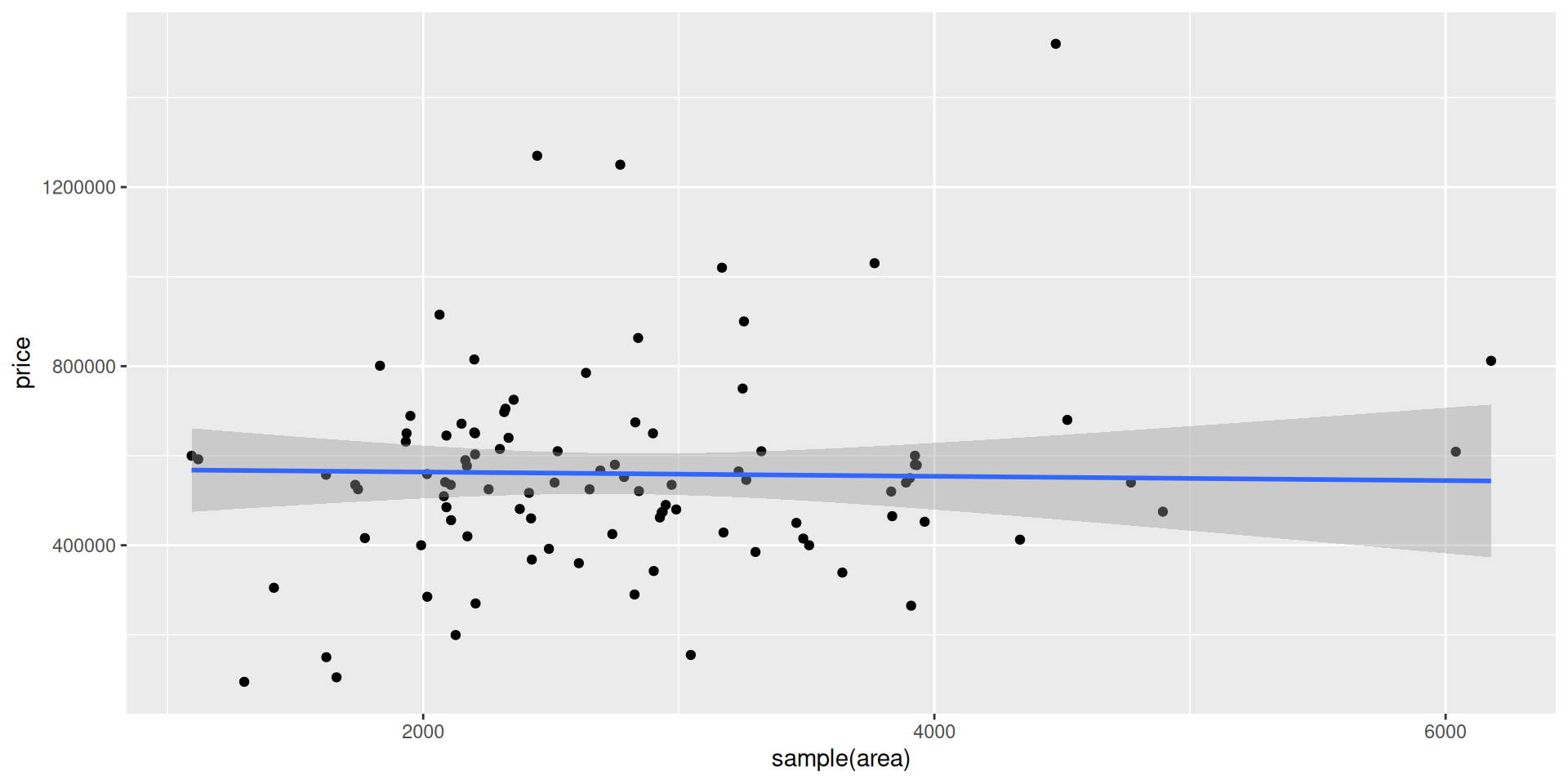
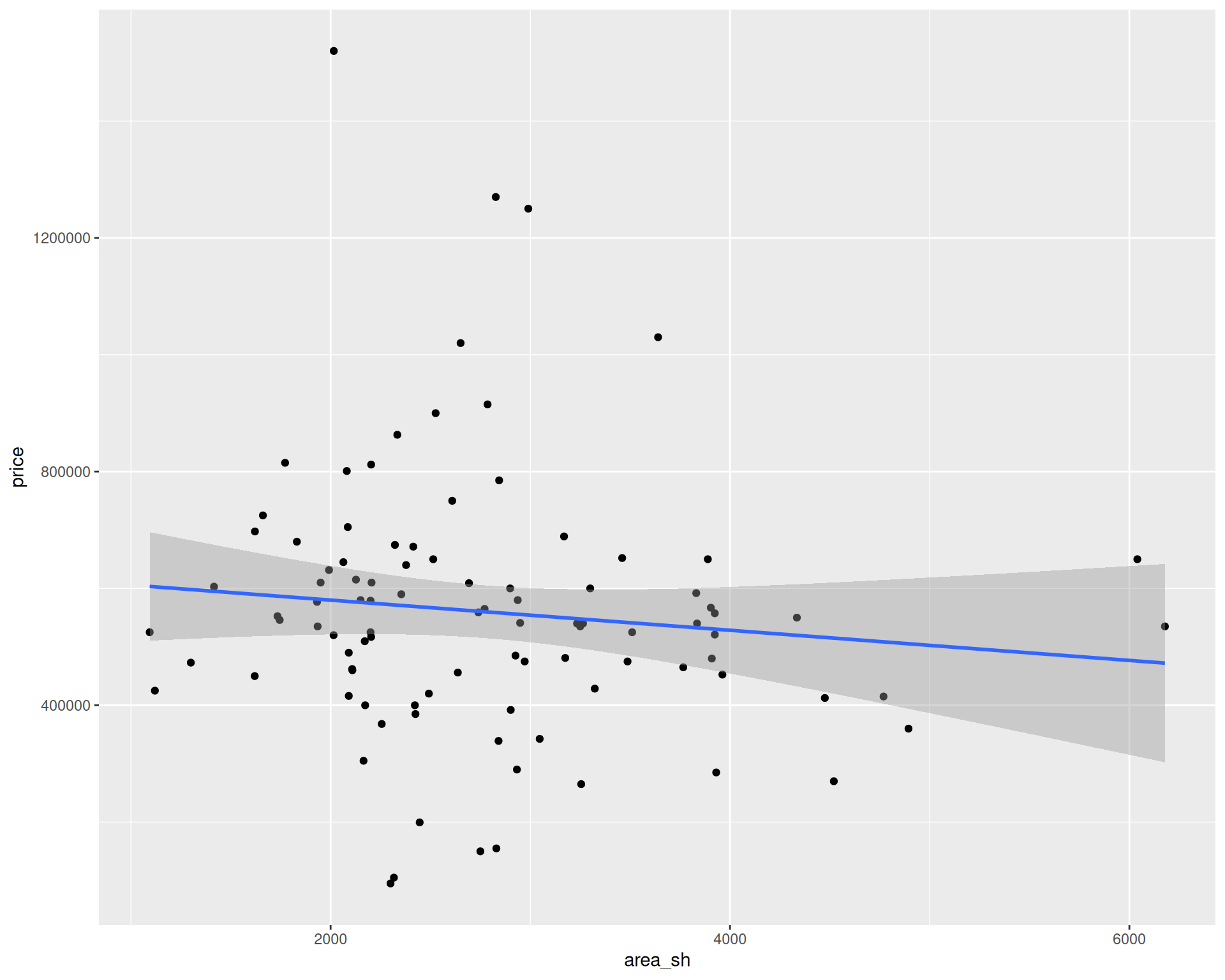
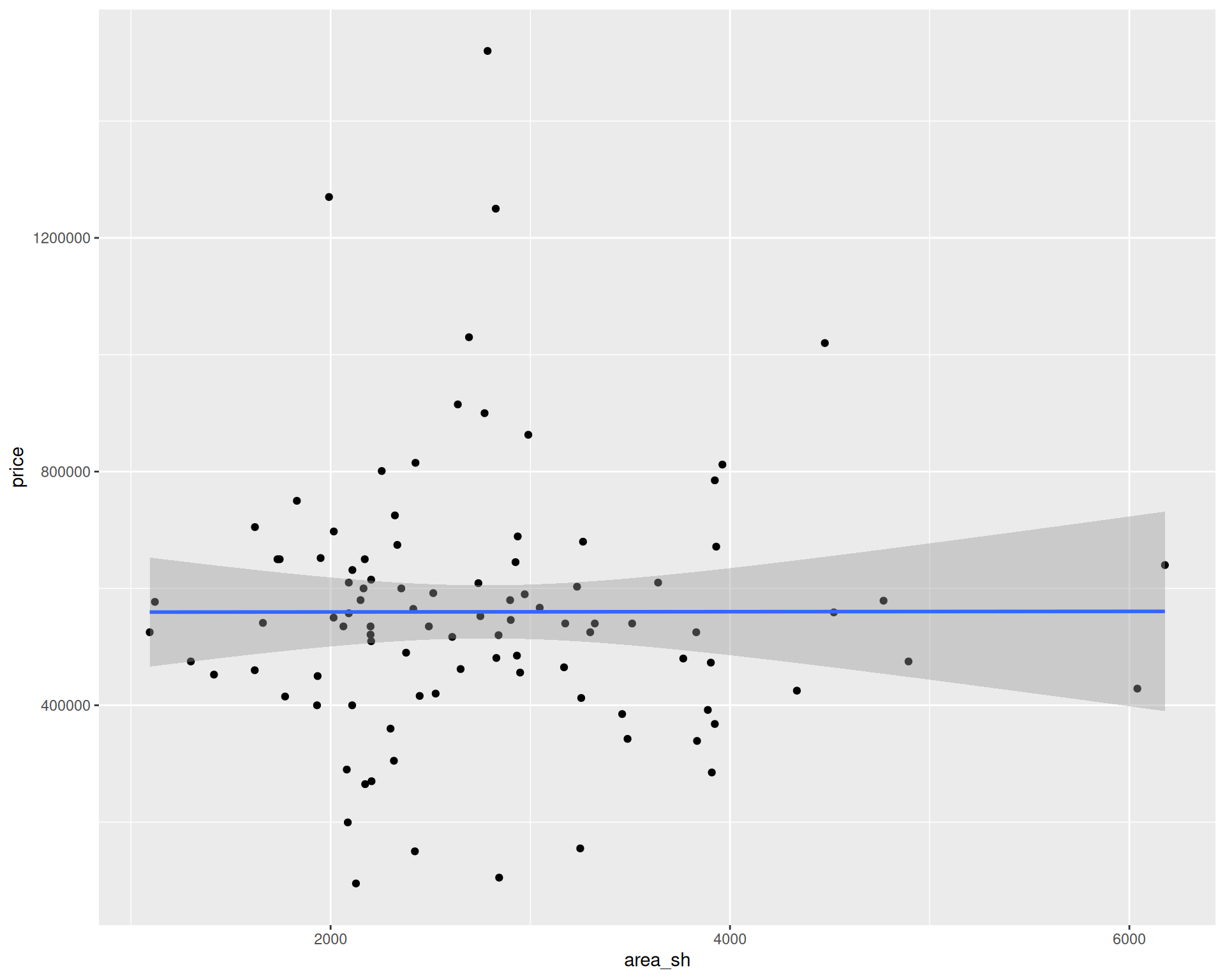
ggplot(duke_forest, aes(x = area, y = price)) +
  geom_point() +
  geom_smooth(method = "lm")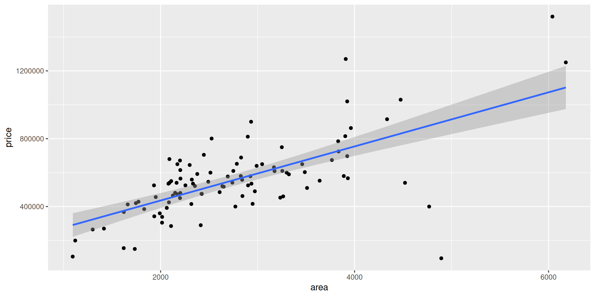
office_cast <- c("Michael Scott", "Jim Halpert", "Pam Beesly", "Dwight Schrute")
office_cast
[1] "Michael Scott" "Jim Halpert" "Pam Beesly"
[4] "Dwight Schrute". . .
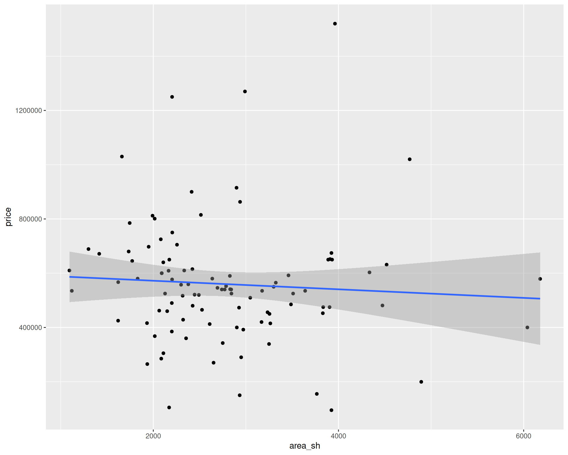
# A tibble: 2 × 2
  term        estimate
  <chr>          <dbl>
1 (Intercept) 603842.
2 area_sh        -15.8
# A tibble: 2 × 2
  term        estimate
  <chr>          <dbl>
1 (Intercept) 631641.
2 area_sh        -25.8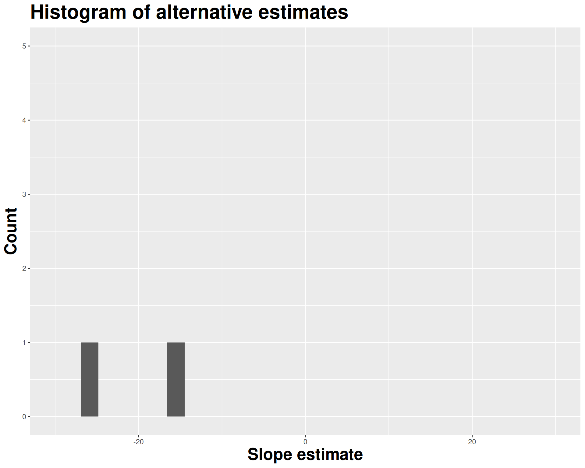
# A tibble: 2 × 2
  term          estimate
  <chr>            <dbl>
1 (Intercept) 559207.
2 area_sh          0.249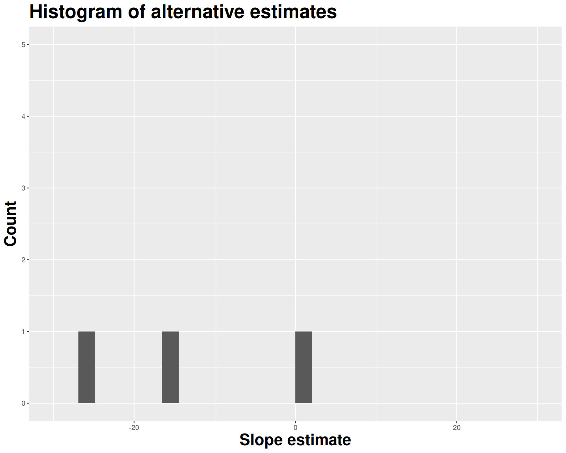
null_dist# A tibble: 2,000 × 3
# Groups: replicate [1,000]
replicate term estimate
<int> <chr> <dbl>
1 1 intercept 551475.
2 1 area 3.03
3 2 intercept 478969.
4 2 area 29.1
5 3 intercept 581602.
6 3 area -7.81
7 4 intercept 492889.
8 4 area 24.1
9 5 intercept 484819.
10 5 area 27.0
# ℹ 1,990 more rowsnull_dist |>
filter(term == "area") |>
ggplot(aes(x = estimate)) +
geom_histogram(binwidth = 15)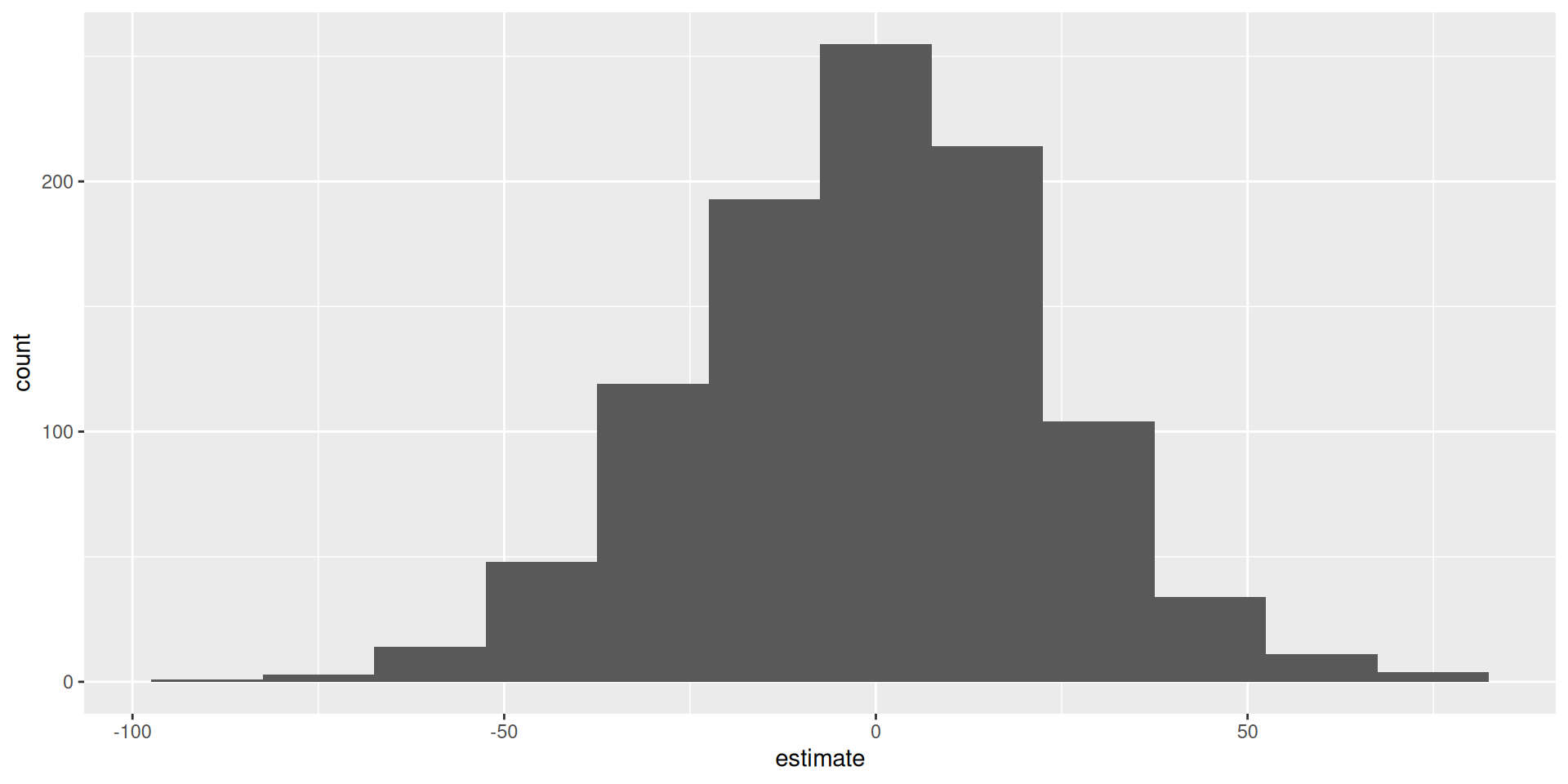
visualize(null_dist) +
  shade_p_value(obs_stat = observed_fit, direction = "two-sided")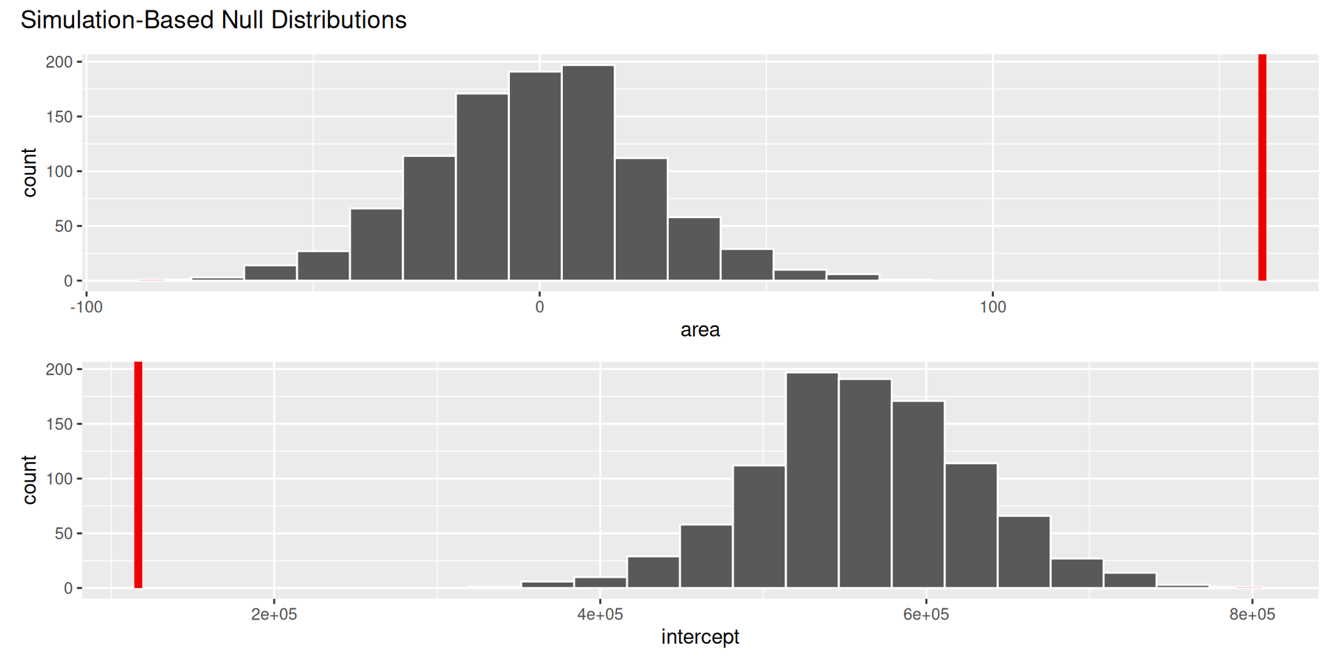
null_dist |>
  get_p_value(obs_stat = observed_fit, direction = "two-sided")
Warning: Please be cautious in reporting a p-value of 0. This result is an
approximation based on the number of `reps` chosen in the
`generate()` step.
ℹ See `get_p_value()` (`?infer::get_p_value()`) for more information.
Please be cautious in reporting a p-value of 0. This result is an
approximation based on the number of `reps` chosen in the
`generate()` step.
ℹ See `get_p_value()` (`?infer::get_p_value()`) for more information.# A tibble: 2 × 2
term p_value
<chr> <dbl>
1 area 0
2 intercept 0Based on the p-value calculated, what is the conclusion of the hypothesis test?
\(H_0\) person innocent vs \(H_A\) person guilty
\(H_0\) person well vs \(H_A\) person sick.
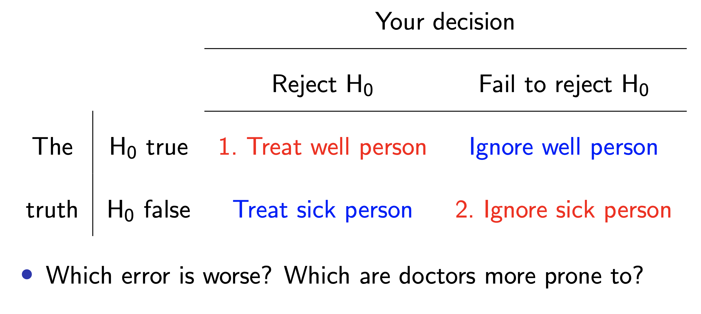
Pick a threshold \(\alpha\in[0,\,1]\) called the discernibility level (you may also hear it called the significance level) and threshold the \(p\)-value:
Unless otherwise specified, we will use a discernibility level \(\alpha = 0.05\); you may see this worded as “What is your conclusion at the 5% discernibility level?” or functionally similar