Final Study Guide

The final exam is cumulative, but there will be a greater emphasis on material covered in the second half of the course (i.e., statistical modeling and inference). For a review of material covered in the first half of the course, please reference the “Midterm Review” provided here.

Try this

Attempt all of the problems below without resources. Make note of your pain points and blind spots along the way. That might give you an idea of the stuff you would benefit from if you had it on a cheat sheet.

Concepts and main ideas

Question 1

Can you answer each of these in one or two sentences?

When we plot a line of best fit for a numerical predictor and numerical response, what does “best” mean?
What does the correlation coefficient between two numerical variables measure?
What does the $R^2$ of a linear regression measure?
What is the difference between $Y=\beta_0+\beta_1 X + \varepsilon$ and $\widehat{Y}=b_0+b_1 X$?
Under what circumstances is the intercept in a regression model a “meaningful” quantity?
If you run a “simple” linear regression model with a numerical response and a categorical predictor with three levels, what does the computer actually do to estimate that model?
Consider this bit of toy code: linear_reg() |> fit(_BLANK_, df)? What goes in the blank? What purpose does that argument serve, and how do you use it?
Let $\widehat{y}^{(\text{old})}$ be the prediction at $x$ of a simple linear regression, and let $\widehat{y}^{(\text{new})}$ be the prediction at $x+1$ of the same regression. How are $\widehat{y}^{(\text{old})}$ and $\widehat{y}^{(\text{new})}$ related? In other words, how do the predictions of the simple linear regression model differ when you change the input from $x$ to $x+1$?
Let $\widehat{o}^{(\text{old})}$ be the estimated odds at $x$ from a simple logistic regression model, and let $\widehat{o}^{(\text{new})}$ be the estimated odds at $x+1$ of the same regression. How are $\widehat{o}^{(\text{old})}$ and $\widehat{o}^{(\text{new})}$ related? In other words, how do the predicted odds of the simple logistic regression model differ when you change the input from $x$ to $x+1$?
Why is adjusted $R^2$ a better linear regression model selection criterion than unadjusted $R^2$?

Visual understanding

Question 2

Here’s a nonsense dataset that I made up:

Rows: 65
Columns: 3
$ x     <dbl> 4.892947, 4.232442, 1.892767, 4.730670, 5.373811, 4.156704, 4.44…
$ y     <dbl> 8.197365, 39.317266, 9.828075, 18.352456, 20.915403, 19.258701, …
$ color <fct> forestgreen, blue, forestgreen, red, red, red, blue, red, forest…

Imagine you run this code:

The output would be a lil’ table like this:

`term`	`estimate`
`(Intercept)`	$b_0$
`x`	$b_1$
`colorblue`	$b_2$
`colorforestgreen`	$b_3$

A plot of the model fit might look something like this:

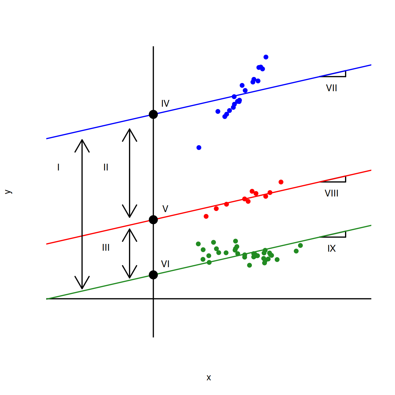
Match the labeled features of the plot to the correct quantity listed below:

$b_0$
$b_1$
$b_2$
$b_3$
$b_0 + b_1$
$b_0 + b_2$
$b_0 + b_3$
$b_1 + b_2$
$b_1 + b_3$
$b_2 + b_3$
$b_2 - b_3$

Note: Some of these quantities might go unused, and some might be used more than once.

Questions 3 - 8

In what follows, let $y$ be a binary response, let $x$ be a numerical predictor, and let $z$ be a binary predictor. Match the S-curve to the model equation.

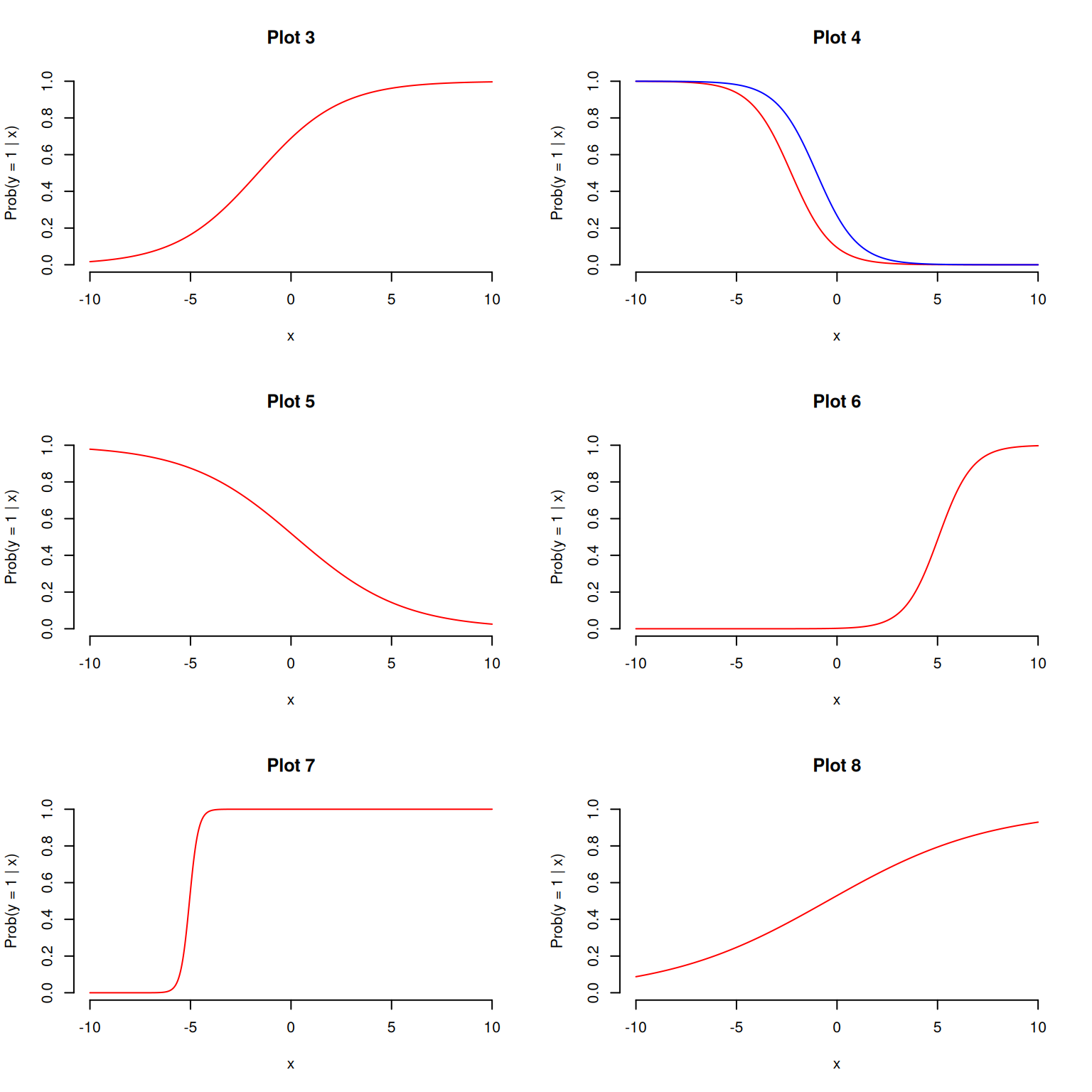
$\log\left(\frac{\hat{p}}{1-\hat{p}}\right) = 22.9 + 4.54 \times x$
$\log\left(\frac{\hat{p}}{1-\hat{p}}\right) = 0.118 + 0.246 \times x$
$\log\left(\frac{\hat{p}}{1-\hat{p}}\right) = 0.798 + 0.486 \times x$
$\log\left(\frac{\hat{p}}{1-\hat{p}}\right) = -6.035 + 1.194 \times x$
$\log\left(\frac{\hat{p}}{1-\hat{p}}\right) = -2.26 - 0.99 \times x+1.26\times z$
$\log\left(\frac{\hat{p}}{1-\hat{p}}\right) = 0.079 -0.373 \times x$

Questions 9 - 12

Recall the dataset on spam emails:

email

# A tibble: 3,921 × 21
   spam  exclaim_mess to_multiple from     cc sent_email time               
   <fct>        <dbl> <fct>       <fct> <int> <fct>      <dttm>             
 1 0                0 0           1         0 0          2012-01-01 06:16:41
 2 0                1 0           1         0 0          2012-01-01 07:03:59
 3 0                6 0           1         0 0          2012-01-01 16:00:32
 4 0               48 0           1         0 0          2012-01-01 09:09:49
 5 0                1 0           1         0 0          2012-01-01 10:00:01
 6 0                1 0           1         0 0          2012-01-01 10:04:46
 7 0                1 1           1         0 1          2012-01-01 17:55:06
 8 0               18 1           1         1 1          2012-01-01 18:45:21
 9 0                1 0           1         0 0          2012-01-01 21:08:59
10 0                0 0           1         0 0          2012-01-01 18:12:00
# ℹ 3,911 more rows
# ℹ 14 more variables: image <dbl>, attach <dbl>, dollar <dbl>, winner <fct>,
#   inherit <dbl>, viagra <dbl>, password <dbl>, num_char <dbl>,
#   line_breaks <int>, format <fct>, re_subj <fct>, exclaim_subj <dbl>,
#   urgent_subj <fct>, number <fct>

Here is a regression model trained on all available predictors:

log_fit <- logistic_reg() |>
  fit(spam ~ ., data = email)

The in-sample predictions of the model are here:

email_aug <- augment(log_fit, email)
email_aug

# A tibble: 3,921 × 24
   .pred_class .pred_0  .pred_1 spam  exclaim_mess to_multiple from     cc
   <fct>         <dbl>    <dbl> <fct>        <dbl> <fct>       <fct> <int>
 1 0             0.867 1.33e- 1 0                0 0           1         0
 2 0             0.943 5.70e- 2 0                1 0           1         0
 3 0             0.942 5.78e- 2 0                6 0           1         0
 4 0             0.920 7.96e- 2 0               48 0           1         0
 5 0             0.903 9.74e- 2 0                1 0           1         0
 6 0             0.901 9.87e- 2 0                1 0           1         0
 7 0             1.000 7.89e-12 0                1 1           1         0
 8 0             1.000 1.24e-12 0               18 1           1         1
 9 0             0.862 1.38e- 1 0                1 0           1         0
10 0             0.922 7.76e- 2 0                0 0           1         0
# ℹ 3,911 more rows
# ℹ 16 more variables: sent_email <fct>, time <dttm>, image <dbl>,
#   attach <dbl>, dollar <dbl>, winner <fct>, inherit <dbl>, viagra <dbl>,
#   password <dbl>, num_char <dbl>, line_breaks <int>, format <fct>,
#   re_subj <fct>, exclaim_subj <dbl>, urgent_subj <fct>, number <fct>

To see how well the model did, we can compute the classification error rates for different thresholds and summarize the results with the ROC curve:

email_roc <- roc_curve(email_aug, truth = spam, .pred_1, event_level = "second")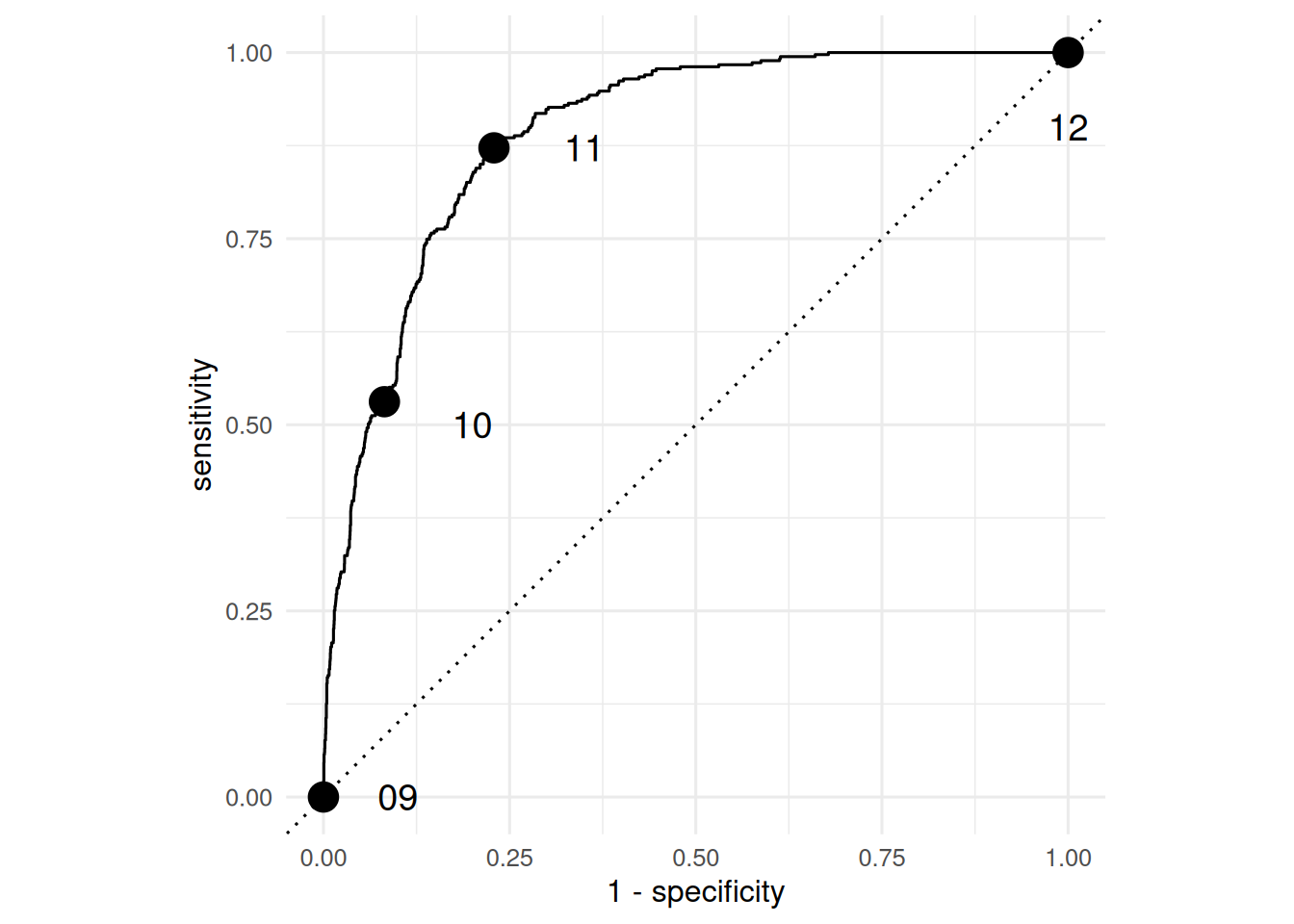

Match the point on the ROC curve to the threshold that was used to compute it.

email_aug |>
  mutate(.pred_class = if_else(.pred_1 <= 0.25, 0, 1)) |>
  count(spam, .pred_class) |> group_by(spam) |> mutate(prop = n / sum(n))

# A tibble: 4 × 4
# Groups:   spam [2]
  spam  .pred_class     n   prop
  <fct>       <dbl> <int>  <dbl>
1 0               0  3263 0.918 
2 0               1   291 0.0819
3 1               0   172 0.469 
4 1               1   195 0.531

email_aug |>
  mutate(.pred_class = if_else(.pred_1 <= 0.0, 0, 1)) |>
  count(spam, .pred_class) |> group_by(spam) |> mutate(prop = n / sum(n))

# A tibble: 2 × 4
# Groups:   spam [2]
  spam  .pred_class     n  prop
  <fct>       <dbl> <int> <dbl>
1 0               1  3554     1
2 1               1   367     1

email_aug |>
  mutate(.pred_class = if_else(.pred_1 <= 1.00, 0, 1)) |>
  count(spam, .pred_class) |> group_by(spam) |> mutate(prop = n / sum(n))

# A tibble: 2 × 4
# Groups:   spam [2]
  spam  .pred_class     n  prop
  <fct>       <dbl> <int> <dbl>
1 0               0  3554     1
2 1               0   367     1

email_aug |>
  mutate(.pred_class = if_else(.pred_1 <= 0.1, 0, 1)) |>
  count(spam, .pred_class) |> group_by(spam) |> mutate(prop = n / sum(n))

# A tibble: 4 × 4
# Groups:   spam [2]
  spam  .pred_class     n  prop
  <fct>       <dbl> <int> <dbl>
1 0               0  2740 0.771
2 0               1   814 0.229
3 1               0    47 0.128
4 1               1   320 0.872

Stat doctor

What’s wrong with the interpretations below? Diagnose the problem and fix it if possible.

Question 13

Some bozo ran this regression and wrote the following interpretation:

linear_reg() |>
  fit(bill_length_mm ~ flipper_length_mm, penguins) |>
  tidy()

# A tibble: 2 × 5
  term              estimate std.error statistic  p.value
  <chr>                <dbl>     <dbl>     <dbl>    <dbl>
1 (Intercept)         -7.26     3.20       -2.27 2.38e- 2
2 flipper_length_mm    0.255    0.0159     16.0  1.74e-43

If the flipper length of a penguin increases by 1mm, then the bill length will increase by 0.25mm.

Question 14

Some schmuck ran this regression and wrote the following interpretation:

logistic_reg() |>
  fit(spam ~ num_char, email) |>
  tidy()

# A tibble: 2 × 5
  term        estimate std.error statistic   p.value
  <chr>          <dbl>     <dbl>     <dbl>     <dbl>
1 (Intercept)  -1.80     0.0716     -25.1  2.04e-139
2 num_char     -0.0621   0.00801     -7.75 9.50e- 15

If the number of characters in an email increases by 1000, then the estimated probability of that email being spam is lower by -0.062, on average.

FYI: from the documentation (?email), num_char is “The number of characters in the email, in thousands.”

Question 15

Some putz ran this regression and wrote the following interpretation:

linear_reg() |>
  fit(body_mass_g ~ flipper_length_mm + bill_length_mm, penguins) |> 
  tidy()

# A tibble: 3 × 5
  term              estimate std.error statistic  p.value
  <chr>                <dbl>     <dbl>     <dbl>    <dbl>
1 (Intercept)       -5737.      308.      -18.6  7.80e-54
2 flipper_length_mm    48.1       2.01     23.9  7.56e-75
3 bill_length_mm        6.05      5.18      1.17 2.44e- 1

If flipper length and bill length both increase by 1mm, then we predict that body mass is lower by 48.14 grams, on average.

Question 16

Some blockhead ran this regression and wrote the following interpretation:

linear_reg() |>
  fit(body_mass_g ~ flipper_length_mm * species, penguins) |>
  tidy()

# A tibble: 6 × 5
  term                               estimate std.error statistic  p.value
  <chr>                                 <dbl>     <dbl>     <dbl>    <dbl>
1 (Intercept)                        -2536.      879.      -2.88  4.19e- 3
2 flipper_length_mm                     32.8       4.63     7.10  7.69e-12
3 speciesChinstrap                    -501.     1523.      -0.329 7.42e- 1
4 speciesGentoo                      -4251.     1427.      -2.98  3.11e- 3
5 flipper_length_mm:speciesChinstrap     1.74      7.86     0.222 8.25e- 1
6 flipper_length_mm:speciesGentoo       21.8       6.94     3.14  1.84e- 3

If the flipper length of a Chinstrap penguin increases by 1mm, then we predict that the body mass is higher by 1.74 grams on average.

Question 17

Some nitwit ran this regression and wrote the following interpretation:

linear_reg() |>
  fit(hp ~ mpg, mtcars) |>
  glance()

# A tibble: 1 × 12
  r.squared adj.r.squared sigma statistic     p.value    df logLik   AIC   BIC
      <dbl>         <dbl> <dbl>     <dbl>       <dbl> <dbl>  <dbl> <dbl> <dbl>
1     0.602         0.589  43.9      45.5 0.000000179     1  -165.  337.  341.
# ℹ 3 more variables: deviance <dbl>, df.residual <int>, nobs <int>

About 60% of the observed variation in miles/gallon is explained by the model.

Question 18

Some chooch ran this regression and wrote the following interpretation:

logistic_reg() |>
  fit(spam ~ exclaim_mess + viagra + dollar, email) |>
  tidy()

# A tibble: 4 × 5
  term         estimate std.error statistic p.value
  <chr>           <dbl>     <dbl>     <dbl>   <dbl>
1 (Intercept)  -2.22      0.0568   -39.1    0      
2 exclaim_mess  0.00189   0.00108    1.75   0.0794 
3 viagra        1.86     40.6        0.0459 0.963  
4 dollar       -0.0656    0.0208    -3.15   0.00165

If an email contains no exclamation marks, no dollar signs, and no mentions of viagra, then the model predicts that the probability of it being spam is $e^{-2.218}\approx 0.10886$.

Question 19

Some nincompoop ran this regression and wrote the following interpretation:

linear_reg() |>
  fit(bill_length_mm ~ bill_depth_mm + sex, penguins) |>
  tidy()

# A tibble: 3 × 5
  term          estimate std.error statistic  p.value
  <chr>            <dbl>     <dbl>     <dbl>    <dbl>
1 (Intercept)      61.0      2.35      26.0  7.39e-82
2 bill_depth_mm    -1.15     0.141     -8.16 7.35e-15
3 sexmale           5.44     0.555      9.81 4.18e-20

If a male penguin has a bill depth of 0mm (sad!), then we expect its bill length to be 60.99mm on average.

Question 20

Some silly goose ran this regression and wrote the following interpretation:

linear_reg() |>
  fit(body_mass_g ~ flipper_length_mm + bill_length_mm, penguins) |>
  glance()

# A tibble: 1 × 12
  r.squared adj.r.squared sigma statistic   p.value    df logLik   AIC   BIC
      <dbl>         <dbl> <dbl>     <dbl>     <dbl> <dbl>  <dbl> <dbl> <dbl>
1     0.760         0.759  394.      537. 9.09e-106     2 -2528. 5063. 5079.
# ℹ 3 more variables: deviance <dbl>, df.residual <int>, nobs <int>

The correlation between body mass, flipper length, and bill length is about $\sqrt{0.76}\approx 0.87$.

Pokémon

The data for Questions X - Y was originally gathered using the Complete Pokémon Dataset from Kaggle.

First, let’s load the data:

Rows: 924
Columns: 17
$ name            <chr> "Bulbasaur", "Ivysaur", "Venusaur", "Mega Venusaur", "…
$ generation      <dbl> 1, 1, 1, 1, 1, 1, 1, 1, 1, 1, 1, 1, 1, 1, 1, 1, 1, 1, …
$ type_1          <chr> "Grass", "Grass", "Grass", "Grass", "Fire", "Fire", "F…
$ type_2          <chr> "Poison", "Poison", "Poison", "Poison", NA, NA, "Flyin…
$ height_m        <dbl> 0.7, 1.0, 2.0, 2.4, 0.6, 1.1, 1.7, 1.7, 1.7, 0.5, 1.0,…
$ weight_kg       <dbl> 6.9, 13.0, 100.0, 155.5, 8.5, 19.0, 90.5, 110.5, 100.5…
$ total_points    <dbl> 318, 405, 525, 625, 309, 405, 534, 634, 634, 314, 405,…
$ hp              <dbl> 45, 60, 80, 80, 39, 58, 78, 78, 78, 44, 59, 79, 79, 45…
$ attack          <dbl> 49, 62, 82, 100, 52, 64, 84, 130, 104, 48, 63, 83, 103…
$ defense         <dbl> 49, 63, 83, 123, 43, 58, 78, 111, 78, 65, 80, 100, 120…
$ sp_attack       <dbl> 65, 80, 100, 122, 60, 80, 109, 130, 159, 50, 65, 85, 1…
$ sp_defense      <dbl> 65, 80, 100, 120, 50, 65, 85, 85, 115, 64, 80, 105, 11…
$ speed           <dbl> 45, 60, 80, 80, 65, 80, 100, 100, 100, 43, 58, 78, 78,…
$ catch_rate      <dbl> 45, 45, 45, 45, 45, 45, 45, 45, 45, 45, 45, 45, 45, 25…
$ base_friendship <dbl> 70, 70, 70, 70, 70, 70, 70, 70, 70, 70, 70, 70, 70, 70…
$ base_experience <dbl> 64, 142, 236, 281, 62, 142, 240, 285, 285, 63, 142, 23…
$ is_legendary    <fct> FALSE, FALSE, FALSE, FALSE, FALSE, FALSE, FALSE, FALSE…

Below are several failed attempts at interpreting statistical results for these data. Diagnose the problem and fix it if possible.

Question 21

# A tibble: 2 × 2
  term      estimate
  <chr>        <dbl>
1 intercept  69.7   
2 defense    -0.0144

A Pokémon with speed of 0 will have defense score of 69.66.

Question 22

# A tibble: 4 × 5
  term        estimate std.error statistic  p.value
  <chr>          <dbl>     <dbl>     <dbl>    <dbl>
1 (Intercept)  -7.77     0.609      -12.8  3.07e-37
2 hp            0.0274   0.00423      6.48 8.92e-11
3 attack        0.0230   0.00389      5.92 3.25e- 9
4 defense       0.0162   0.00380      4.25 2.10e- 5

A one unit increase in hp is associated with a 0.027 increase in the probability that the Pokémon is not legendary, on average.

Question 23

# A tibble: 1 × 3
  .metric .estimator .estimate
  <chr>   <chr>          <dbl>
1 roc_auc binary         0.852

About 85% of the variation in the response is explained by the model.

Question 24

# A tibble: 1 × 3
  term    lower_ci upper_ci
  <chr>      <dbl>    <dbl>
1 defense  -0.0657   0.0458

We are confident that 95% of our data lies between -0.065 and 0.046.

Question 25

# A tibble: 2 × 2
  term      p_value
  <chr>       <dbl>
1 defense     0.532
2 intercept   0.532

The probability that the null hypothesis is true (meaning defense and speed are uncorrelated) is about 53%.

Question 26

Because the p-value is greater than 50%, we reject the alternative hypothesis.

Data analysis

Blizzard salaries

In 2020, employees of Blizzard Entertainment circulated a spreadsheet to anonymously share salaries and recent pay increases amidst rising tension in the video game industry over wage disparities and executive compensation. (Source: Blizzard Workers Share Salaries in Revolt Over Pay)

The name of the data frame used for this analysis is blizzard_salary and the variables are:

percent_incr: Raise given in July 2020, as percent increase with values ranging from 1 (1% increase) to 21.5 (21.5% increase)
salary_type: Type of salary, with levels Hourly and Salaried
annual_salary: Annual salary, in USD, with values ranging from $50,939 to $216,856.
performance_rating: Most recent review performance rating, with levels Poor, Successful, High, and Top. The Poor level is the lowest rating and the Top level is the highest rating.

The first ten rows of blizzard_salary are shown below:

# A tibble: 409 × 4
   percent_incr salary_type annual_salary performance_rating
          <dbl> <chr>               <dbl> <chr>             
 1          1   Salaried               1  High              
 2          1   Salaried               1  Successful        
 3          1   Salaried               1  High              
 4          1   Hourly             33987. Successful        
 5         NA   Hourly             34798. High              
 6         NA   Hourly             35360  <NA>              
 7         NA   Hourly             37440  <NA>              
 8          0   Hourly             37814. <NA>              
 9          4   Hourly             41101. Top               
10          1.2 Hourly             42328  <NA>              
# ℹ 399 more rows

Question 27

You fit a model for predicting raises (percent_incr) from salaries (annual_salary). We’ll call this model raise_1_fit. A tidy output of the model is shown below.

# A tibble: 2 × 5
  term           estimate  std.error statistic   p.value
  <chr>             <dbl>      <dbl>     <dbl>     <dbl>
1 (Intercept)   1.87      0.432           4.33 0.0000194
2 annual_salary 0.0000155 0.00000452      3.43 0.000669

Which of the following is the best interpretation of the slope coefficient?

For every additional $1,000 of annual salary, the model predicts the raise to be higher, on average, by 1.55%.
For every additional $1,000 of annual salary, the raise goes up by 0.0155%.
For every additional $1,000 of annual salary, the model predicts the raise to be higher, on average, by 0.0155%.
For every additional $1,000 of annual salary, the model predicts the raise to be higher, on average, by 1.87%.

Question 28

You then fit a model for predicting raises (percent_incr) from salaries (annual_salary) and performance ratings (performance_rating). We’ll call this model raise_2_fit. Which of the following is definitely true based on the information you have so far?

Intercept of raise_2_fit is higher than intercept of raise_1_fit.
Slope of raise_2_fit is higher than RMSE of raise_1_fit.
Adjusted $R^2$ of raise_2_fit is higher than adjusted $R^2$ of raise_1_fit.
$R^2$ of raise_2_fit is higher $R^2$ of raise_1_fit.

Question 29

The tidy model output for the raise_2_fit model you fit is shown below.

# A tibble: 5 × 5
  term                            estimate  std.error statistic  p.value
  <chr>                              <dbl>      <dbl>     <dbl>    <dbl>
1 (Intercept)                   3.55       0.508           6.99 1.99e-11
2 annual_salary                 0.00000989 0.00000436      2.27 2.42e- 2
3 performance_ratingPoor       -4.06       1.42           -2.86 4.58e- 3
4 performance_ratingSuccessful -2.40       0.397          -6.05 4.68e- 9
5 performance_ratingTop         2.99       0.715           4.18 3.92e- 5

When your teammate sees this model output, they remark

“The coefficient for performance_ratingSuccessful is negative. That’s weird. I guess it means that people who get successful performance ratings get lower raises.”

How would you respond to your teammate?

Question 30

Ultimately, your teammate decides they don’t like the negative slope coefficients in the model output you created (not that there’s anything wrong with negative slope coefficients!), does something else, and comes up with the following model output.

# A tibble: 5 × 5
  term                            estimate  std.error statistic    p.value
  <chr>                              <dbl>      <dbl>     <dbl>      <dbl>
1 (Intercept)                  -0.511      1.47          -0.347 0.729     
2 annual_salary                 0.00000989 0.00000436     2.27  0.0242    
3 performance_ratingSuccessful  1.66       1.42           1.17  0.242     
4 performance_ratingHigh        4.06       1.42           2.86  0.00458   
5 performance_ratingTop         7.05       1.53           4.60  0.00000644

Unfortunately they didn’t write their code in a Quarto document, instead just wrote some code in the Console and then lost track of their work. They remember using the fct_relevel() function and doing something like the following:

blizzard_salary <- blizzard_salary |>
  mutate(performance_rating = fct_relevel(performance_rating, ___))

What should they put in the blanks to get the same model output as above?

“Poor”, “Successful”, “High”, “Top”
“Successful”, “High”, “Top”
“Top”, “High”, “Successful”, “Poor”
Poor, Successful, High, Top

Question 31

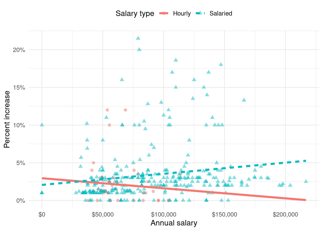
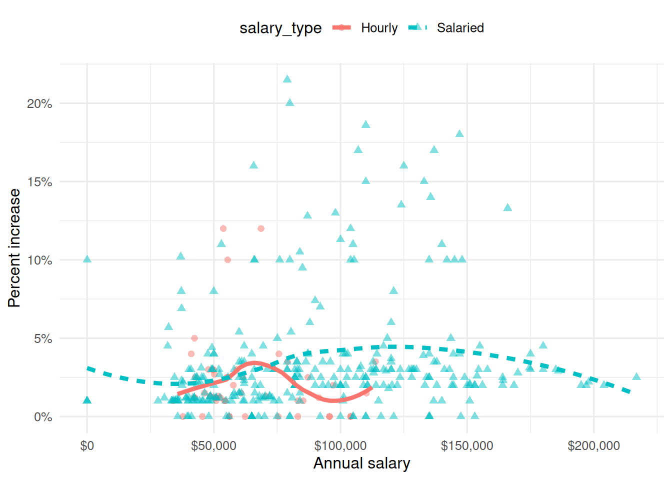
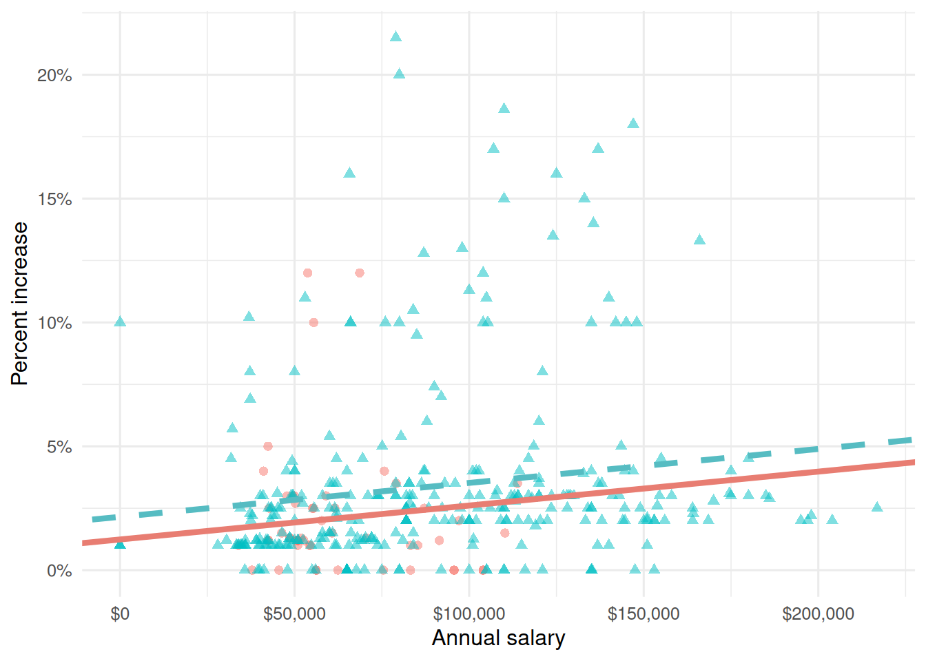
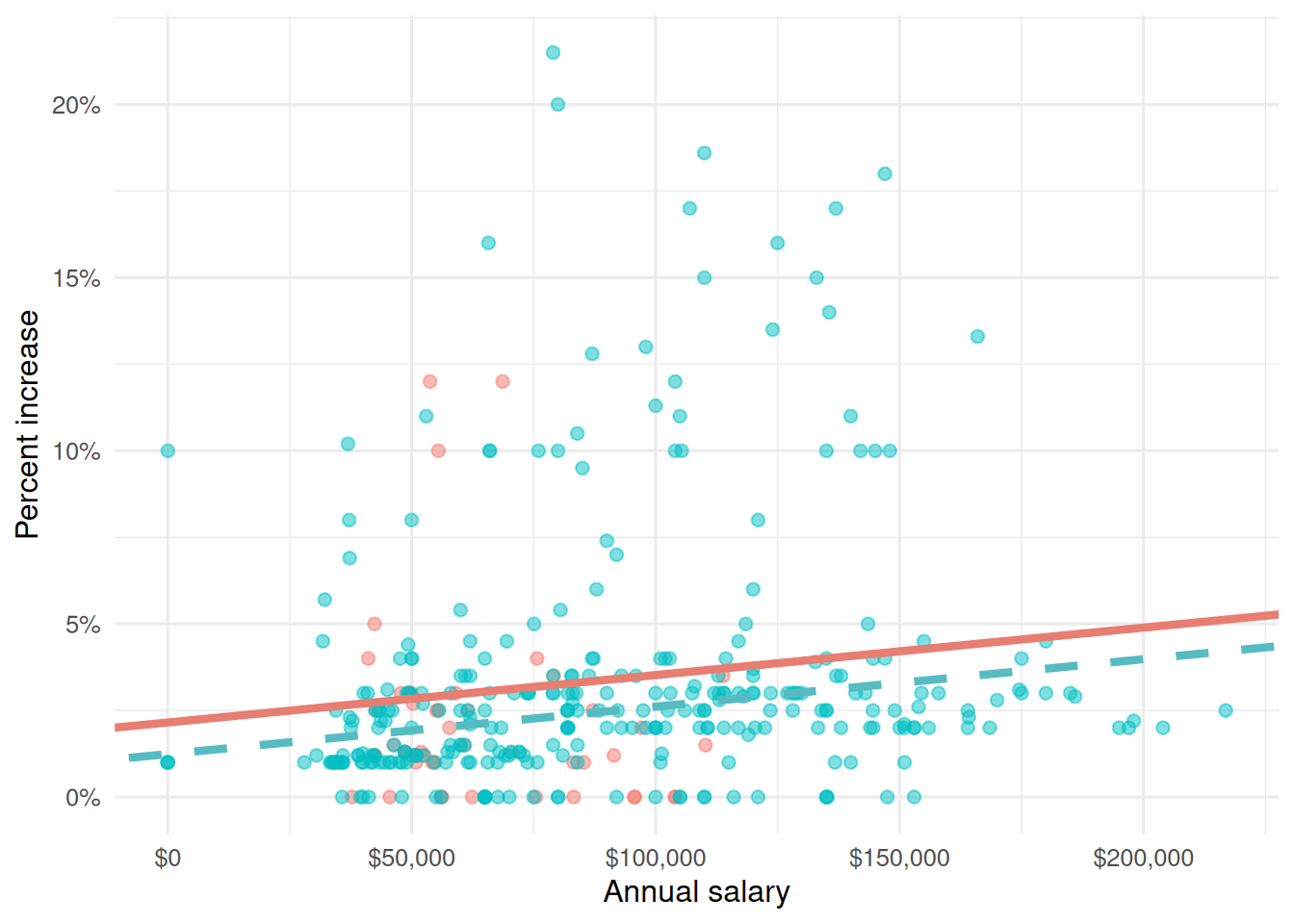
Suppose we fit a model to predict percent_incr from annual_salary and salary_type. A tidy output of the model is shown below.

# A tibble: 3 × 5
  term                 estimate  std.error statistic p.value
  <chr>                   <dbl>      <dbl>     <dbl>   <dbl>
1 (Intercept)         1.24      0.570           2.18 0.0300 
2 annual_salary       0.0000137 0.00000464      2.96 0.00329
3 salary_typeSalaried 0.913     0.544           1.68 0.0938

Which of the following visualizations represent this model? Explain your reasoning.

Question 32

Suppose you now fit a model to predict the natural log of percent increase, log(percent_incr), from performance rating. The model is called raise_4_fit.

You’re provided the following:

tidy(raise_4_fit) |>
  select(term, estimate) |>
  mutate(exp_estimate = exp(estimate))

# A tibble: 4 × 3
  term                         estimate exp_estimate
  <chr>                           <dbl>        <dbl>
1 (Intercept)                     -7.15     0.000786
2 performance_ratingSuccessful     6.93  1025.      
3 performance_ratingHigh           8.17  3534.      
4 performance_ratingTop            8.91  7438.

Based on this, which of the following is true?

a. The model predicts that the percentage increase employees with Successful performance get, on average, is higher by 10.25% compared to the employees with Poor performance rating.

b. The model predicts that the percentage increase employees with Successful performance get, on average, is higher by 6.93% compared to the employees with Poor performance rating.

c. The model predicts that the percentage increase employees with Successful performance get, on average, is higher by a factor of 1025 compared to the employees with Poor performance rating.

d. The model predicts that the percentage increase employees with Successful performance get, on average, is higher by a factor of 6.93 compared to the employees with Poor performance rating.

Movies

The data for this part comes from the Internet Movie Database (IMDB). Specifically, the data are a random sample of movies released between 1980 and 2020.

The name of the data frame used for this analysis is movies, and it contains the variables shown in Table 1.

Table 1: Data dictionary for movies

Variable	Description
`name`	name of the movie
`rating`	rating of the movie (R, PG, etc.)
`genre`	main genre of the movie.
`runtime`	duration of the movie
`year`	year of release
`release_date`	release date (YYYY-MM-DD)
`release_country`	release country
`score`	IMDB user rating
`votes`	number of user votes
`director`	the director
`writer`	writer of the movie
`star`	main actor/actress
`country`	country of origin
`budget`	the budget of a movie (some movies don’t have this, so it appears as 0)
`gross`	revenue of the movie
`company`	the production company

The first thirty rows of the movies data frame are shown in Table 2, with variable types suppressed (since we’ll ask about them later).

\begin{landscape}

Table 2

First 30 rows of movies, with variable types suppressed.

# A tibble: 500 × 16
   name           score runtime genre     rating    release_country release_date
 1 Blue City        4.4 83 mins Action    R         United States   1986-05-02  
 2 Winter Sleep     8.1 196     Drama     Not Rated Turkey          2014-06-12  
 3 Rang De Basan…   8.1 167     Comedy    Not Rated United States   2006-01-26  
 4 Pokémon Detec…   6.6 104     Action    PG        United States   2019-05-10  
 5 A Bad Moms Ch…   5.6 104     Comedy    R         United States   2017-11-01  
 6 Replicas         5.5 107     Drama     PG-13     United States   2019-01-11  
 7 Windy City       5.8 103     Drama     R         Uruguay         1986-01-01  
 8 War for the P…   7.4 140     Action    PG-13     United States   2017-07-14  
 9 Tales from th…   6.4 98      Crime     R         United States   1995-05-24  
10 Fire with Fire   6.5 103     Drama     PG-13     United States   1986-05-09  
11 Raising Helen    6   119     Comedy    PG-13     United States   2004-05-28  
12 Feeling Minne…   5.4 99      Comedy    R         United States   1996-09-13  
13 The Babe         5.9 115     Biography PG        United States   1992-04-17  
14 The Real Blon…   6   105     Comedy    R         United States   1998-02-27  
15 To vlemma tou…   7.6 176     Drama     Not Rated United States   1997-11-01  
16 Going the Dis…   6.3 102     Comedy    R         United States   2010-09-03  
17 Jung on zo       6.8 103     Action    R         Hong Kong       1993-06-24  
18 Rita, Sue and…   6.5 93      Comedy    R         United Kingdom  1987-05-29  
19 Phone Booth      7   81      Crime     R         United States   2003-04-04  
20 Happy Death D…   6.6 96      Comedy    PG-13     United States   2017-10-13  
21 Barely Legal     4.7 90      Comedy    R         Thailand        2006-05-25  
22 Three Kings      7.1 114     Action    R         United States   1999-10-01  
23 Menace II Soc…   7.5 97      Crime     R         United States   1993-05-26  
24 Four Rooms       6.8 98      Comedy    R         United States   1995-12-25  
25 Quartet          6.8 98      Comedy    PG-13     United States   2013-03-01  
26 Tape             7.2 86      Drama     R         Denmark         2002-07-12  
27 Marked for De…   6   93      Action    R         United States   1990-10-05  
28 Congo            5.2 109     Action    PG-13     United States   1995-06-09  
29 Stop-Loss        6.4 112     Drama     R         United States   2008-03-28  
30 Con Air          6.9 115     Action    R         United States   1997-06-06  
# ℹ 470 more rows
# ℹ 9 more variables: budget, gross, votes, year,
#   director, writer, star, company, country

Score vs. runtime

In this part, we fit a model predicting score from runtime and name it score_runtime_fit.

score_runtime_fit <- linear_reg() |>
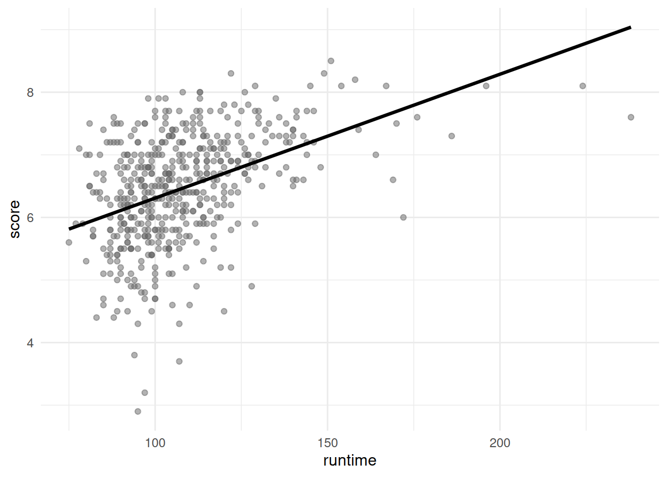
  fit(score ~ runtime, data = movies)

Figure 2 visualizes the relationship between score and runtime as well as the linear model for predicting score from runtime. The first three movies in Table 2 are labeled in the visualization as well. Answer all questions in this part based on Figure 2.

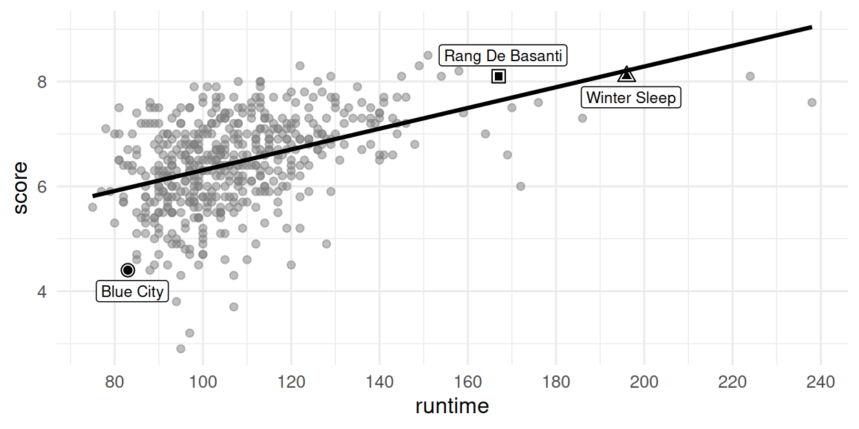
Figure 2: Scatterplot of `score` vs. `runtime` for `movies`.

Question 33

Partial code for producing Figure 2 is given below. Which of the following goes in the blank on Line 2? Select all that apply.

movies |>
  mutate(runtime = ___) |>
  ggplot(aes(x = runtime, y = score)) +
  geom_point(alpha = 0.5) +
  geom_smooth(method = "lm", se = FALSE)
# additional code for annotating Blue City on the plot

grepl(" mins", runtime)
grep(" mins", runtime)
str_remove(runtime, " mins")
as.numeric(str_remove(runtime, " mins"))
na.rm(runtime)

Question 34

Based on this model, order the three labeled movies in Figure 2 in decreasing order of the magnitude (absolute value) of their residuals.

Winter Sleep > Rang De Basanti > Blue City
Winter Sleep > Blue City > Rang De Basanti
Rang De Basanti > Winter Sleep > Blue City
Blue City > Winter Sleep > Rang De Basanti
Blue City > Rang De Basanti > Winter Sleep

Question 35

The R-squared for the model visualized in Figure 2 is 31%. Which of the following is the best interpretation of this value?

31% of the variability in movie runtimes is explained by their scores.
31% of the variability in movie scores is explained by their runtime.
The model accurately predicts scores of 31% of the movies in this sample.
The model accurately predicts scores of 31% of all movies.
The correlation between scores and runtimes of movies is 0.31.

Score vs. runtime or year

The visualizations below show the relationship between score and runtime as well as score and year, respectively. Additionally, the lines of best fit are overlaid on the visualizations.

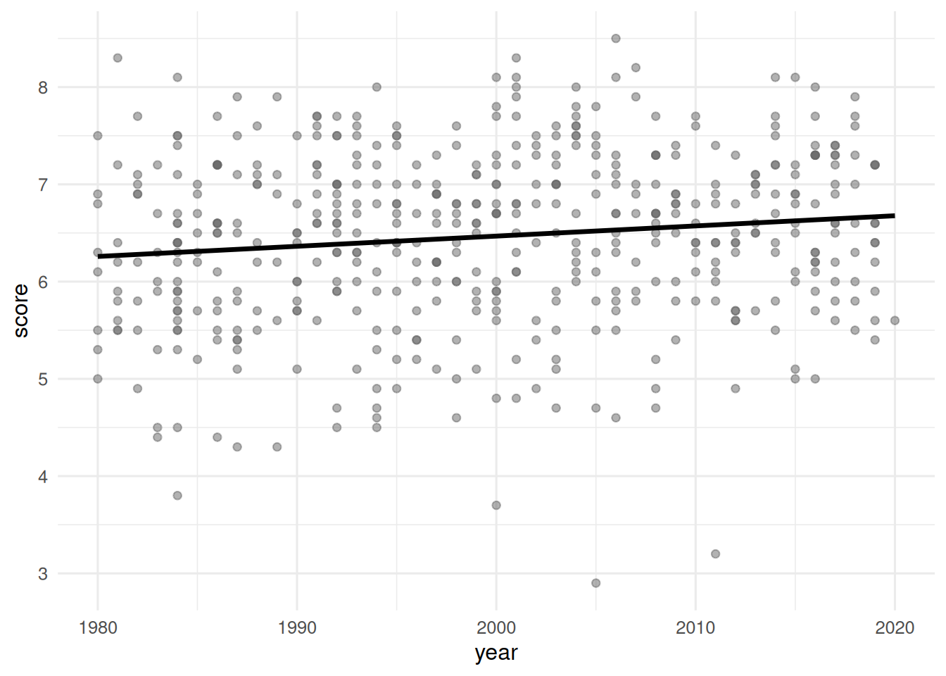
The correlation coefficients of these relationships are calculated below, though some of the code and the output are missing. Answer all questions in this part based on the code and output shown below.

movies |>
  __blank_1__(
    r_score_runtime = cor(runtime, score),
    r_score_year = cor(year, score)
  )

# A tibble: 1 × 2
  r_score_runtime r_score_year
            <dbl>        <dbl>
1           0.434. __blank_2__

Question 36

Which of the following goes in __blank_1__?

summarize
mutate
group_by
arrange
filter

Question 37

What can we say about the value that goes in __blank_2__?

NA
A value between 0 and 0.434.
A value between 0.434 and 1.
A value between 0 and -0.434.
A value between -1 and -0.434.

Score vs. runtime and rating

In this part, we fit a model predicting score from runtime and rating (categorized as G, PG, PG-13, R, NC-17, and Not Rated), and name it score_runtime_rating_fit.

The model output for score_runtime_rating_fit is shown in Table 3. Answer all questions in this part based on Table 3.

Table 3: Regression output for score_runtime_rating_fit.

term	estimate	std.error	statistic	p.value
(Intercept)	4.525	0.332	13.647	0.000
runtime	0.021	0.002	10.702	0.000
ratingPG	-0.189	0.295	-0.642	0.521
ratingPG-13	-0.452	0.292	-1.547	0.123
ratingR	-0.257	0.285	-0.901	0.368
ratingNC-17	-0.355	0.486	-0.730	0.466
ratingNot Rated	-0.282	0.328	-0.860	0.390

Question 38

Which of the following is TRUE about the intercept of score_runtime_rating_fit? Select all that are true.

Keeping runtime constant, G-rated movies are predicted to score, on average, 4.525 points.
Keeping runtime constant, movies without a rating are predicted to score, on average, 4.525 points.
Movies without a rating that are 0 minutes in length are predicted to score, on average, 4.525 points.
All else held constant, movies that are 0 minutes in length are predicted to score, on average, 4.525 points.
G-rated movies that are 0 minutes in length are predicted to score, on average, 4.525 points.

Question 39

Which of the following is the best interpretation of the slope of runtime in score_runtime_rating_fit?

All else held constant, as runtime increases by 1 minute, the score of the movie increases by 0.021 points.
For G-rated movies, all else held constant, as runtime increases by 1 minute, we predict the score of the movie to be higher by 0.021 points on average.
All else held constant, for each additional minute of runtime, movie scores will be higher by 0.021 points on average.
G-rated movies that are 0 minutes in length are predicted to score 0.021 points on average.
For each higher level of rating, the movie scores go up by 0.021 points on average.

Question 40

Fill in the blank:

R-squared for score_runtime_rating_fit (the model predicting score from runtime and rating) _________ the R-squared the model score_runtime_fit (for predicting score from runtime alone).

is less than
is equal to
is greater than
cannot be compared (based on the information provided) to
is both greater than and less than

Question 41

The model score_runtime_rating_fit (the model predicting score from runtime and rating) can be visualized as parallel lines for each level of rating. Which of the following is the equation of the line for R-rated movies?

$\widehat{score} = (4.525 - 0.257) + 0.021 \times runtime$
$score = (4.525 - 0.257) + 0.021 \times runtime$
$\widehat{score} = 4.525 + (0.021 - 0.257) \times runtime$
$score = 4.525 + (0.021 - 0.257) \times runtime$
$\widehat{score} = (4.525 + 0.021) - 0.257 \times runtime$

Holiday movies

A team of five data scientists is working model and make inferences about holiday movies using a dataset on 1835 holiday movies; movies with “holiday”, “Christmas”, “Hanukkah”, or “Kwanzaa” (or variants thereof) in their title. Each member of the team is responsible for a different part of the analysis. The data come from the Internet Movie Database (IMDb). The data frame is called holiday_movies and it contains the variables described in the table below.

Variable	Description
`id`	IMDb ID of movie
`title_type`	Type of the title (Feature Film or TV Movie)
`title`	Title used on promotional materials at the point of release
`year`	Release year of a title
`runtime`	Primary runtime of the title, in minutes
`genre`	Primary genre associated with the title
`score`	Weighted average of all the individual user ratings on IMDb
`num_votes`	Number of votes the title has received on IMDb
`christmas`	Whether the title includes “christmas”, “xmas”, “x mas”, etc.
`hanukkah`	Whether the title includes “hanukkah”, “chanukah”, etc.
`kwanzaa`	Whether the title includes “kwanzaa”
`holiday`	Whether the title includes the word “holiday”

A peek at the data is shown below.

# A tibble: 1,835 × 12
   id        title_type  title     year runtime genre  score num_votes christmas
   <chr>     <chr>       <chr>    <dbl>   <dbl> <chr>  <dbl>     <dbl> <lgl>    
 1 tt0020356 Feature Fi… Sailor'…  1929      58 Comedy   5.4        55 FALSE    
 2 tt0020823 Feature Fi… The Dev…  1930      80 Drama    6         242 FALSE    
 3 tt0020985 Feature Fi… Holiday   1930      91 Comedy   6.3       638 FALSE    
 4 tt0021268 Feature Fi… Holiday…  1930      83 Comedy   7.4       256 FALSE    
 5 tt0021377 Feature Fi… Sin Tak…  1930      81 Comedy   6.1       740 FALSE    
 6 tt0021381 Feature Fi… Sinners…  1930      60 Other    6.3       688 FALSE    
 7 tt0023039 Feature Fi… Husband…  1931      70 Drama    6.4        27 FALSE    
 8 tt0024869 Feature Fi… Beggar'…  1934      60 Other    5.6        15 FALSE    
 9 tt0025006 Feature Fi… Cowboy …  1934      56 Other    4.8        74 FALSE    
10 tt0025037 Feature Fi… Death T…  1934      79 Drama    6.9      2361 FALSE    
# ℹ 1,825 more rows
# ℹ 3 more variables: hanukkah <lgl>, kwanzaa <lgl>, holiday <lgl>

Question 42

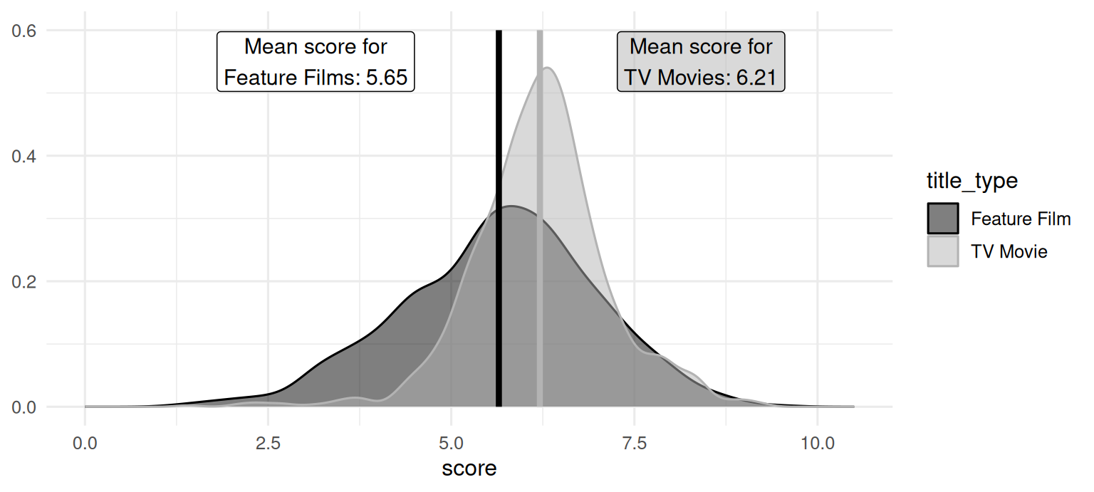
The second team member is working on inference, focusing on comparing scores between Feature Films and TV Movies using the full dataset. They use the full dataset for their analysis. Answer the questions in this part for this team member’s portion of the analysis.

The density curves below show the distributions of scores in Feature Films and TV Movies. The means are overlaid on these distributions: a mean score of 5.65 for Feature Films and a mean score of 6.21 for TV Movies. The observed difference between these scores (TV Movies - Feature Films) is 0.56.

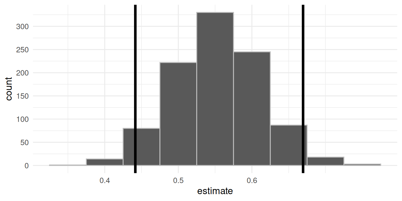
A bootstrap distribution of the difference between the mean scores of holiday TV Movies and Feature Films is generated using the code below:

The plot below visualizes the bootstrap distribution. The 95% confidence interval is (0.442, 0.670). The bounds for this interval are overlaid on the plot.

Noting that this guide is written in Quarto with all figures and tables produced with code, which of the following is TRUE about this analysis? Select all that apply.

We are 95% confident that 44.2% to 67% of holiday movies are TV Movies.
The upper bound of the interval marks the 2.5th percentile of the bootstrap distribution.
We are 95% confident that the mean score of holiday TV Movies is 0.442 points to 0.67 points higher than holiday Feature Films.
If this document is rendered again, we might get slightly different values for the bounds of the confidence interval.
1,000 bootstrap samples were taken when constructing this confidence interval.

Question 43

A post in a data science blog states that holiday TV movies score discernibly differently than holiday Feature Films, on average. Suppose you want to evaluate this claim using a hypothesis test so you write the following code to simulate the null distribution.

The plot below visualizes the null distributions for the slope and intercept. Focus on the slope.

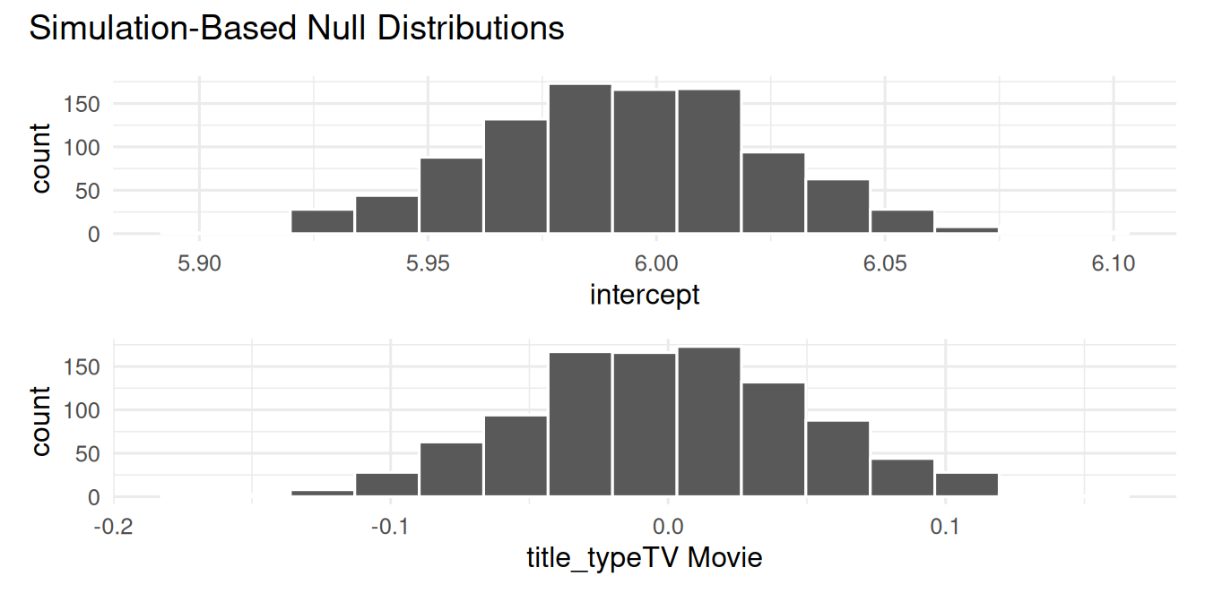
Which of the following is TRUE about this analysis? Select all that apply.

The null hypothesis states that the mean score of all holiday TV movies is equal to the mean score of all holiday Feature Films.
The alternative hypothesis states that the mean score of all holiday TV movies is different than the mean score of all holiday Feature Films.
The p-value is approximately 0.
The data provide discernible evidence that the mean score of all holiday TV movies is equal to the mean score of all holiday Feature Films.
The confidence interval from the previous question and the result of the hypothesis test in this question do not agree with each other.

Question 44

The third team member is working on modeling, predicting score. They first split up the data into training and testing sets.

They then fit a model predicting score from runtime and genre (categorized as Comedy, Drama, Other, Animation, Family, and Romance), and name it score_runtime_genre_fit, using the training data. Answer the questions in this part for this team member’s portion of the analysis.

The model output for score_runtime_genre_fit is shown below.

term	estimate	std.error	statistic	p.value
(Intercept)	7.327	0.258	28.360	0.000
runtime	-0.018	0.006	-3.183	0.001
genreComedy	-1.001	0.369	-2.714	0.007
genreDrama	-1.177	0.506	-2.327	0.020
genreFamily	-0.086	0.497	-0.172	0.863
genreOther	-0.609	0.331	-1.841	0.066
genreRomance	1.216	1.580	0.770	0.442
runtime:genreComedy	0.012	0.006	1.928	0.054
runtime:genreDrama	0.018	0.007	2.377	0.018
runtime:genreFamily	0.000	0.008	0.064	0.949
runtime:genreOther	0.008	0.006	1.264	0.206
runtime:genreRomance	-0.012	0.019	-0.644	0.520

Which of the following is true about the intercept of score_runtime_genre_fit? Select all that apply.

The intercept is meaningless in context of the data.
Animation movies that are 0 minutes in length are predicted to score, on average, 7.327 points.
All else held constant, movies that are 0 minutes in length are predicted to score, on average, 7.327 points.
Movies without a genre that are 0 minutes in length are predicted to score, on average, 7.327 points.
Keeping runtime constant, animation movies are predicted to score, on average, 7.327 points.

Question 45

Fill in the blank:

Adjusted R-squared for score_runtime_genre_fit (the model predicting score from runtime and genre) _________ the adjusted R-squared of the model score_runtime_fit (for predicting score from runtime alone).

is equal to
is less than
is greater than
is both greater than and less than
cannot be compared (based on the information provided) to

Question 46

The fourth team member is also working on modeling, but they classifying movies as either Feature Films or TV Movies (title_type) based on their runtime, score, and num_votes. Their code and output is shown below.

# A tibble: 4 × 3
  title_type   .pred_class      n
  <fct>        <fct>        <int>
1 TV Movie     TV Movie       256
2 TV Movie     Feature Film    30
3 Feature Film TV Movie        95
4 Feature Film Feature Film    78

Which of the following is the false positive rate of the model for this testing set?

30 / (30 + 256) = 0.1
256 / (30 + 256) = 0.9
95 / (95 + 78) = 0.55
78 / (95 + 78) = 0.45
78 / (30 + 78) = 0.72

Question 47

Suppose you fit one other model, predicting title_type from runtime and score only. You should choose this model over the original model if …

it has a higher adjusted R-squared
it has a higher R-squared
it has a lower false positive rate
it has a higher false negative rate
it has a higher area under the ROC curve