ggplot(mtcars, aes(x = wt, y = mpg)) +
  geom_point() +
  geom_smooth(method = "lm")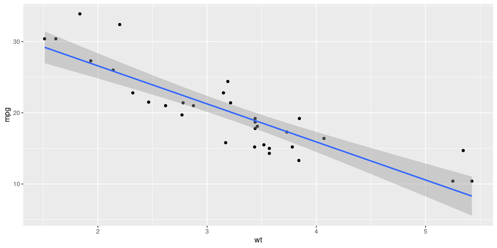
Lecture 20
This is an idealized representation of the data: \[ y = \beta_0+\beta_1x +\varepsilon; \]
There is some “true line” floating out there with a “true slope” \(\beta_1\) and “true intercept” \(\beta_0\);
With infinite amounts of perfectly measured data, we could know \(\beta_0\) and \(\beta_1\) exactly;
We don’t have that, so we must use finite amounts of imperfect data to estimate;
We are especially interested in \(\beta_1\) because is characterizes the association between \(x\) and \(y\), which is useful for prediction.
\(\beta_1\) is an unknown quantity we are trying to learn about using noisy, imperfect data. Learning comes in three flavors:
POINT ESTIMATION: get a single-number best guess for \(\beta_1\);
INTERVAL ESTIMATION: get a range of likely values for \(\beta_1\) that characterizes (sampling) uncertainty;
HYPOTHESIS TESTING: use the data to evaluate competing claims about \(\beta_1\).
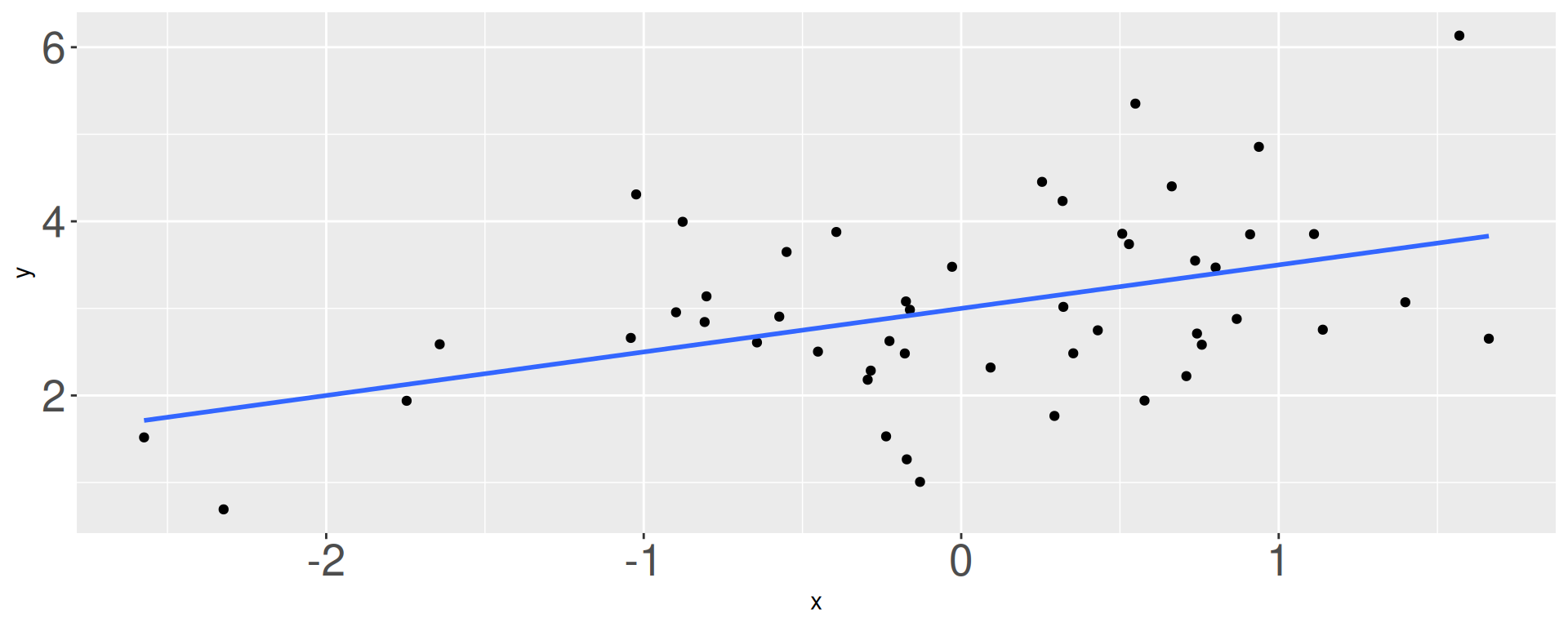
We estimate \(\beta_0\) and \(\beta_1\) with the coefficients of the best fit line:
\[ \widehat{y}=b_0+b_1x. \]
“Best” means “least squares.” We pick the estimates so that the sum of squared residuals is as small as possible. Play around!
ggplot(mtcars, aes(x = wt, y = mpg)) +
geom_point() +
geom_smooth(method = "lm")
linear_reg() |>
  fit(mpg ~ wt, data = mtcars) |>
  tidy()
# A tibble: 2 × 5
term estimate std.error statistic p.value
<chr> <dbl> <dbl> <dbl> <dbl>
1 (Intercept) 37.3 1.88 19.9 8.24e-19
2 wt -5.34 0.559 -9.56 1.29e-10How do our point estimates vary across alternative, hypothetical datasets?
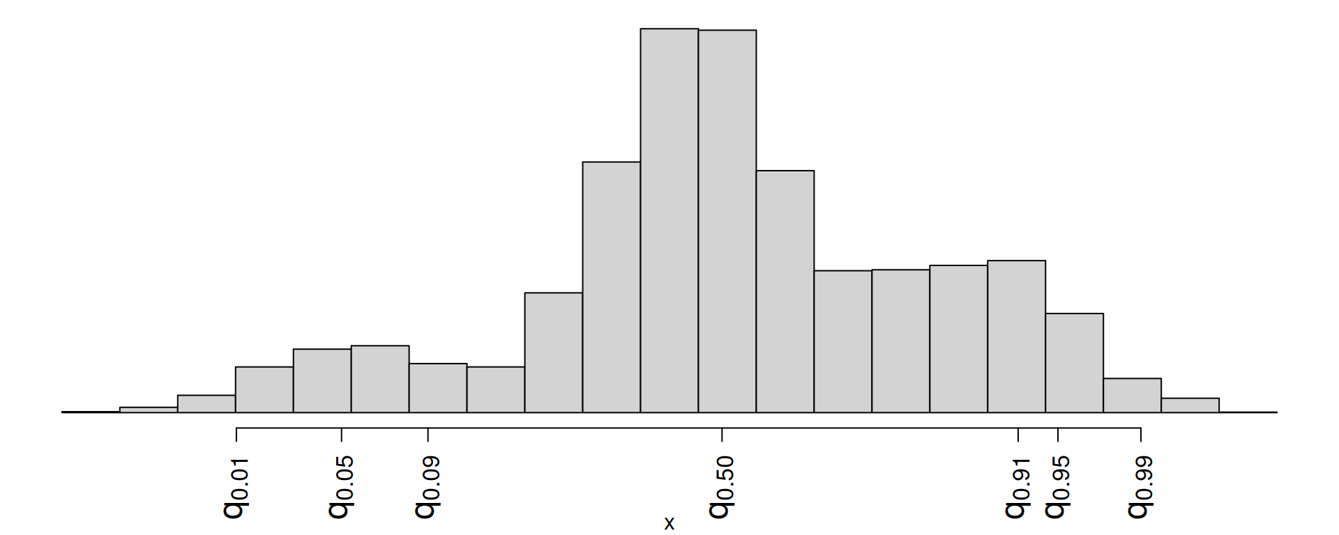
We can use the bootstrap to construct alternative datasets and assess the sensitivity of our estimates to changes in the data.
This histogram displays variation in the slope estimate across alternative datasets.
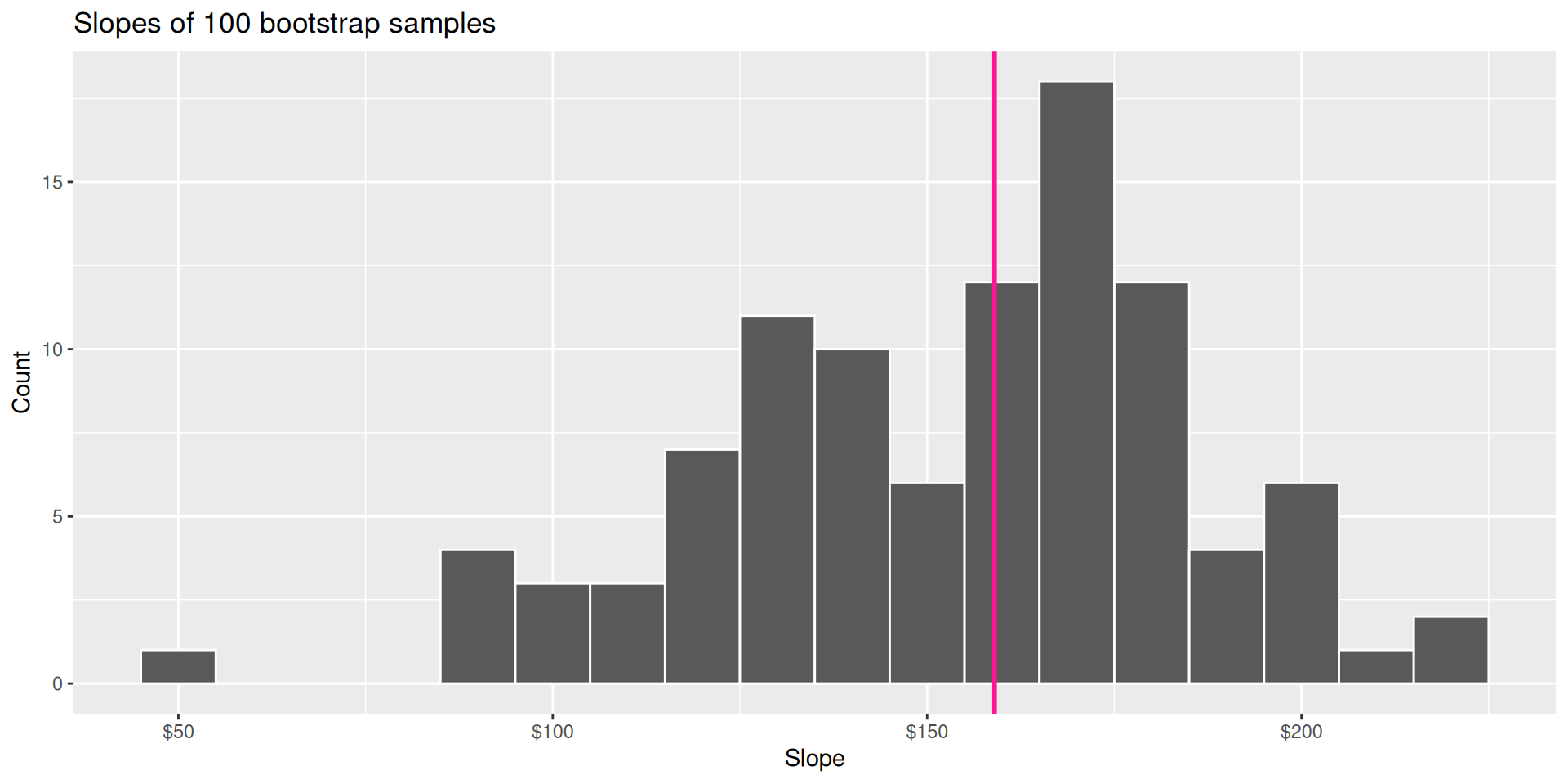
Pick a range that swallows up a large % of the histogram:
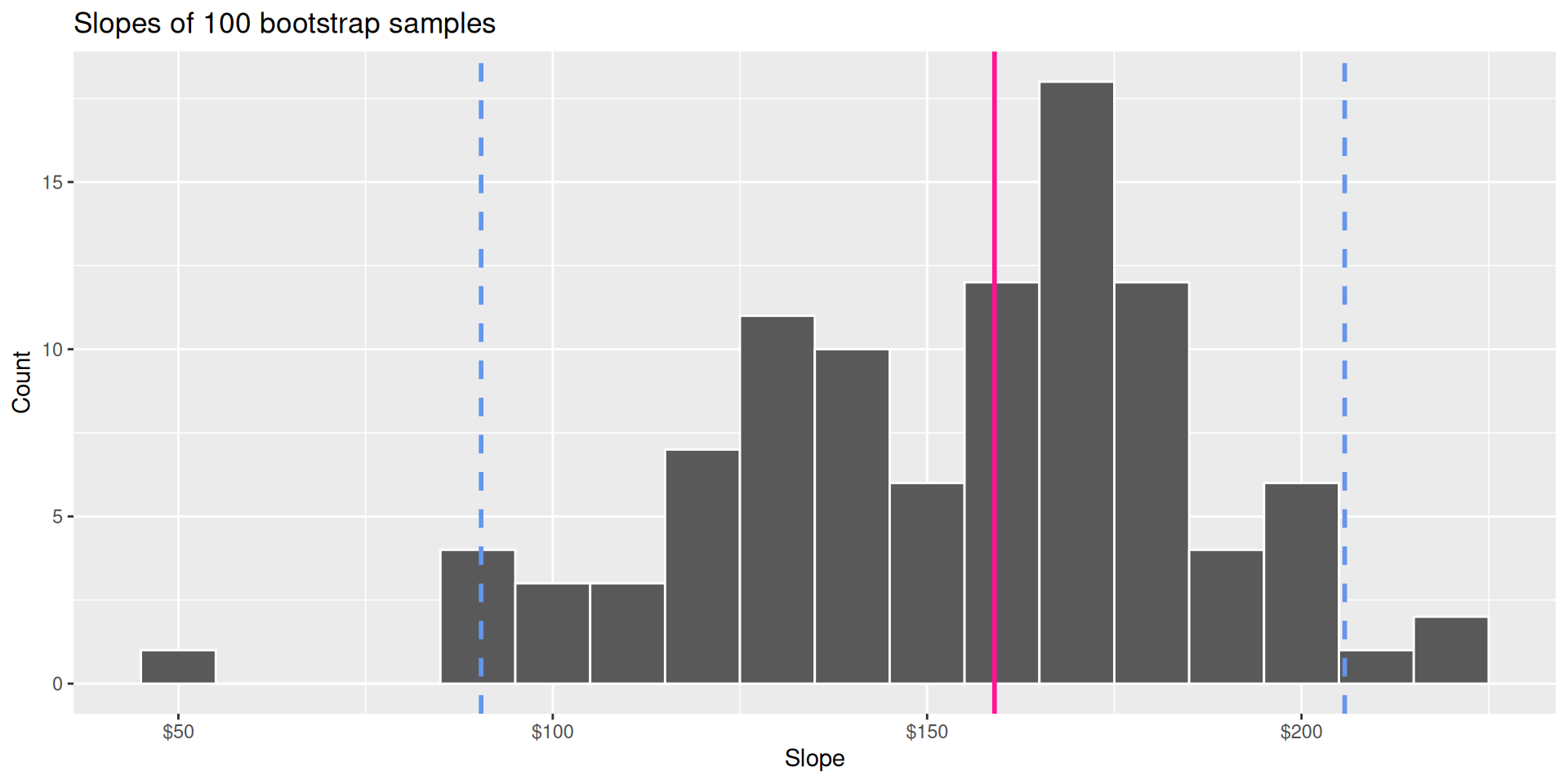
We use quantiles (think IQR), but there are other ways.
Two competing claims about \(\beta_1\): \[ \begin{aligned} H_0&: \beta_1=0\quad(\text{nothing going on})\\ H_A&: \beta_1\neq0\quad(\text{something going on}) \end{aligned} \]
In words: “is there sufficient evidence that x and y are correlated, or not?”
Do the data strongly favor one or the other?
How can we quantify this?
Think hypothetically: if the null hypothesis were in fact true, would my results be out of the ordinary?
My results represent the reality of actual data. If they conflict with the null, then you throw out the null and stick with reality;
How do we quantify “would my results be out of the ordinary”?
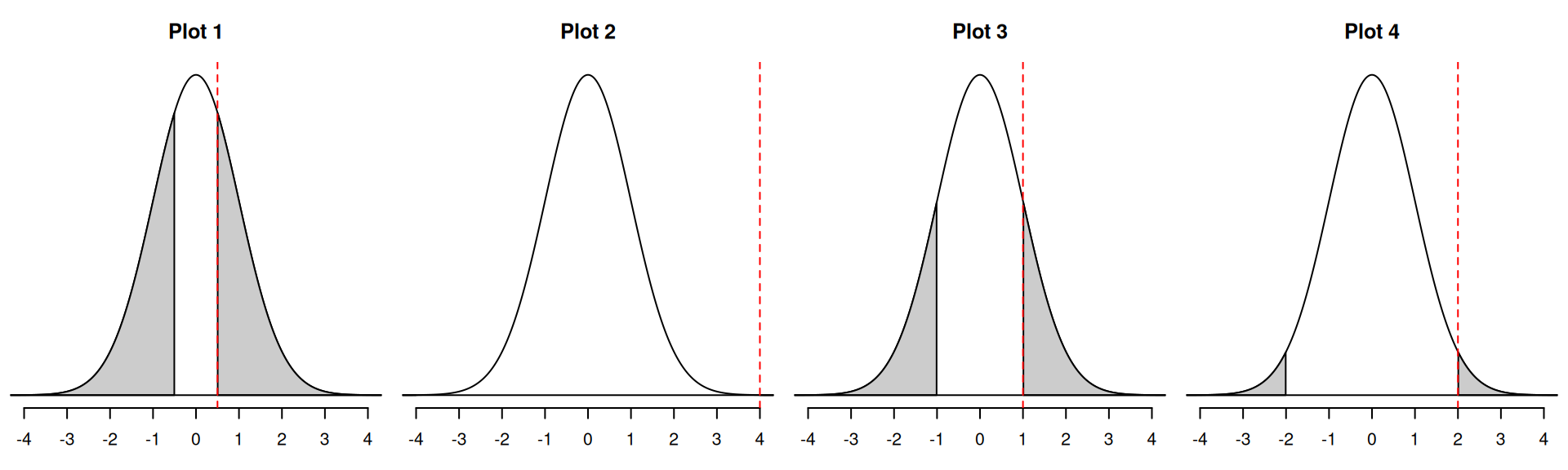
If the null happened to be true, how would we expect our results to vary across datasets? We can use simulation to answer this:
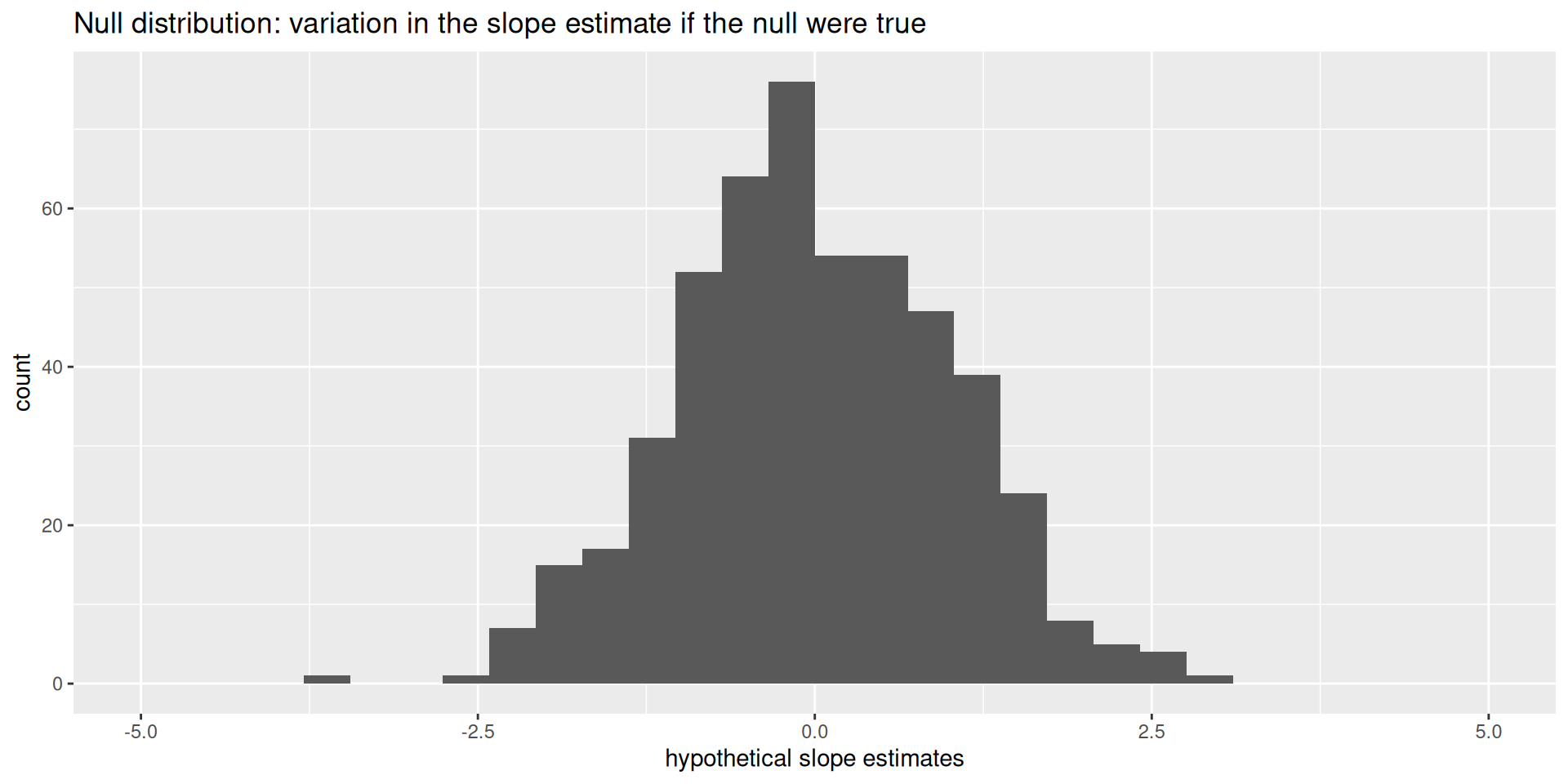
This is how the world should look if the null is true.
Locate the actual results of your actual data analysis under the null distribution. Are they in the middle? Are they in the tails?
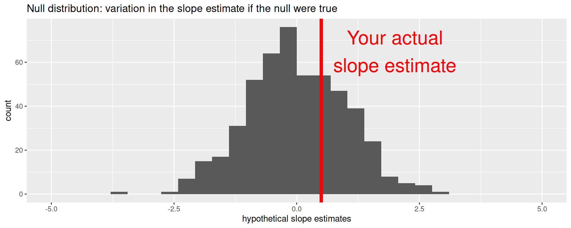
Are these results in harmony or conflict with the null?
Locate the actual results of your actual data analysis under the null distribution. Are they in the middle? Are they in the tails?
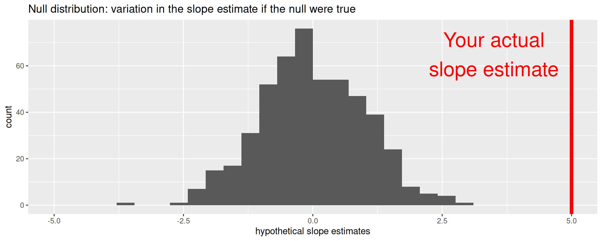
Are these results in harmony or in conflict with the null?
Locate the actual results of your actual data analysis under the null distribution. Are they in the middle? Are they in the tails?
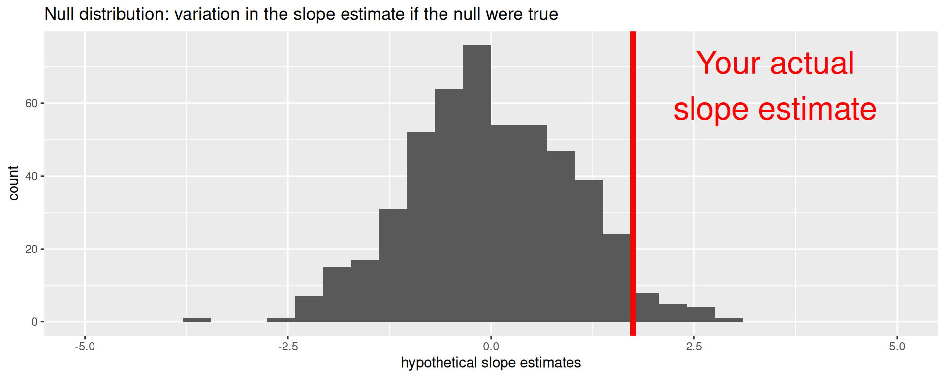
Are these results in harmony or in conflict with the null?
What is a p-value?
The \(p\)-value is the probability of being even farther out in the tails of the null distribution than your results already were.
if this number is very low, then your results would be out of the ordinary if the null were true, so maybe the null was never true to begin with;
if this number is high, then your results may be perfectly compatible with the null.
p-value is the fraction of the histogram area shaded red:
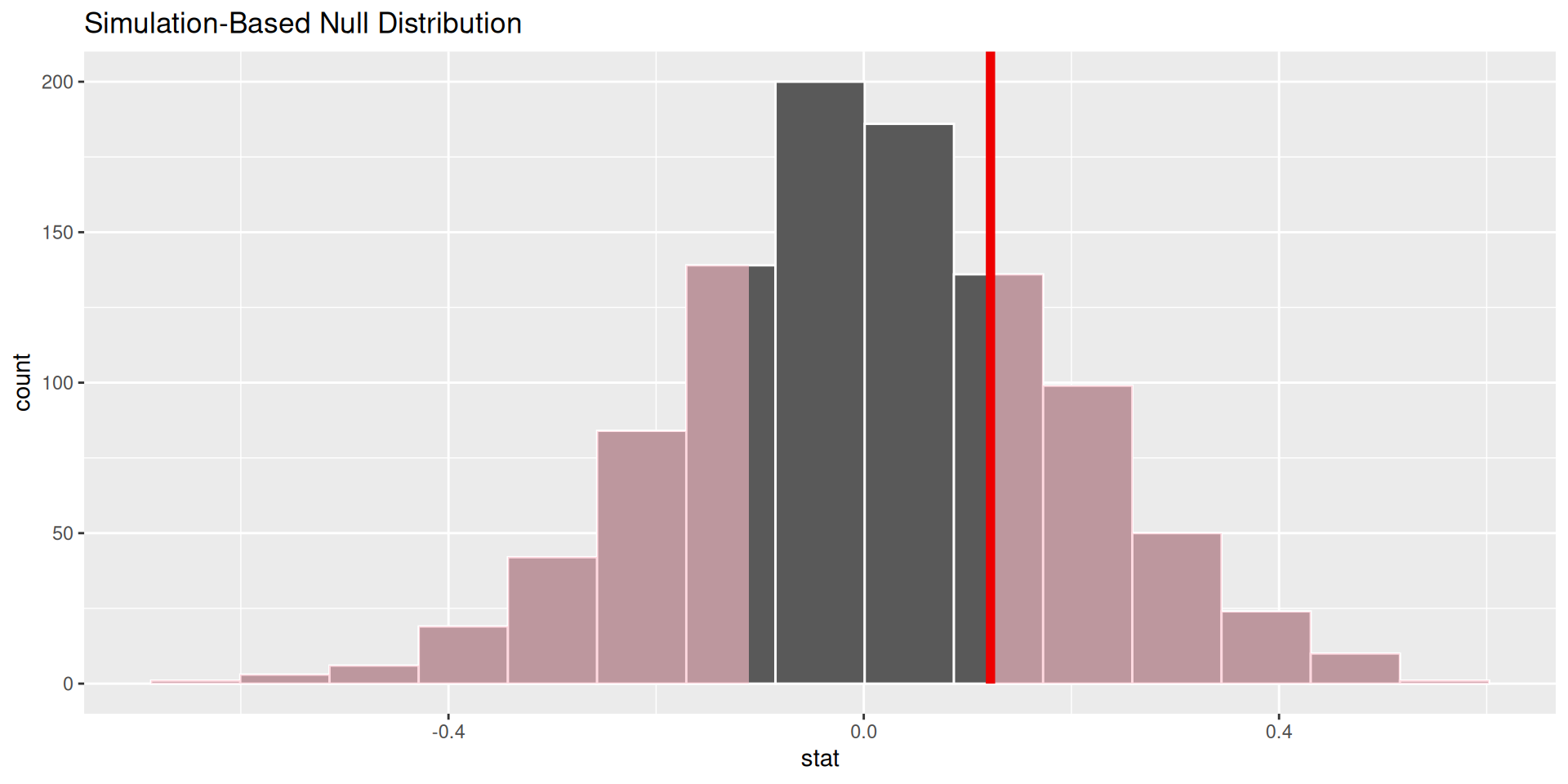
. . .
Big ol’ p-value. Null remains plausible
p-value is the fraction of the histogram area shaded red:
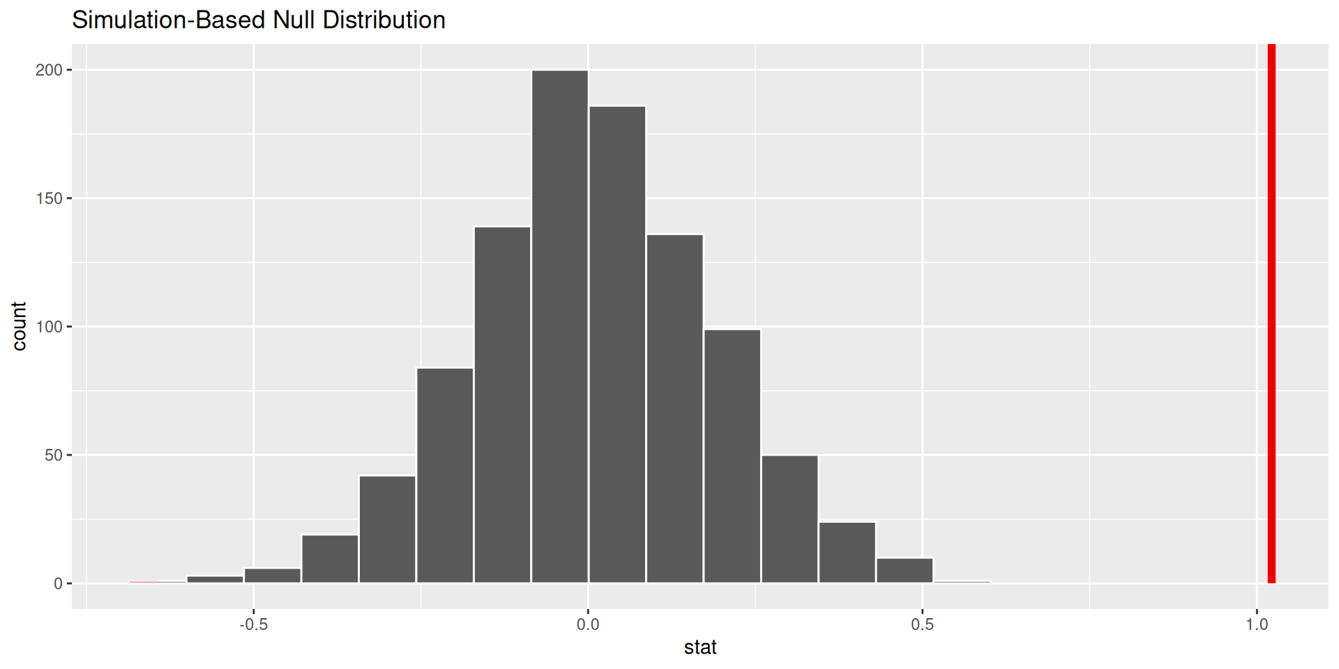
. . .
p-value is basically zero. Null looks bogus.
p-value is the fraction of the histogram area shaded red:
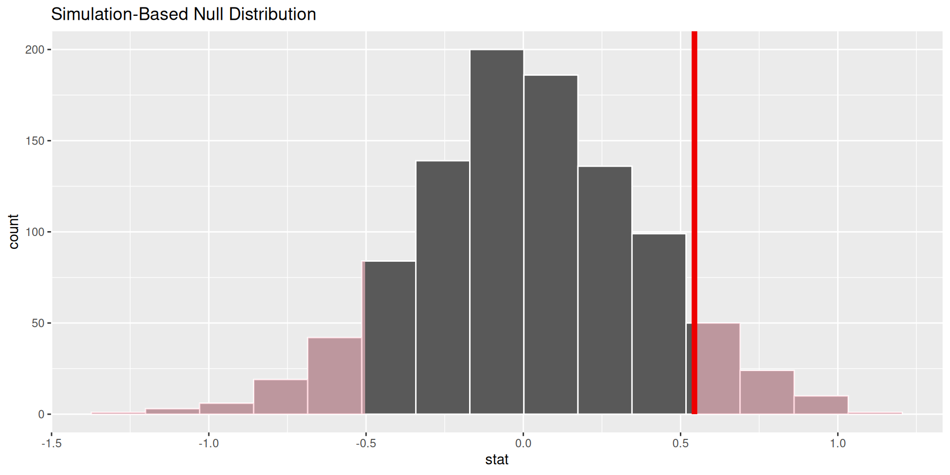
. . .
p-value is…kinda small? Null looks…?
How do we decide if the p-value is big enough or small enough?
Pick a threshold \(\alpha\in[0,\,1]\) called the discernibility level:
Standard choices: \(\alpha=0.01, 0.05, 0.1, 0.15\).

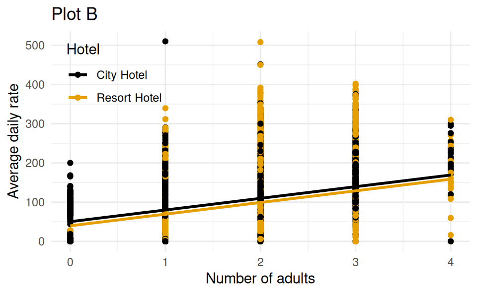
The following model predicts adr from adults and hotel type. Which of the following is the best interpretation of the slope coefficient for adults?
# A tibble: 3 × 5
  term              estimate std.error statistic   p.value
  <chr>                <dbl>     <dbl>     <dbl>     <dbl>
1 (Intercept)           50.2     0.606      82.8 0
2 adults                29.7     0.312      95.4 0
3 hotelResort Hotel    -10.6     0.323     -32.8 6.78e-235
“For each additional adult in the booking, the average daily rate is predicted to be higher by $29.00…”
. . .
on average, holding hotel type constant.
for Resort Hotels compared to City Hotels, on average.
for City Hotels compared to Resort Hotels, on average.
on average, not holding any other variables constant.
Which of the following is the correct interpretation of the slope coefficient for hotel?
# A tibble: 3 × 5
  term              estimate std.error statistic   p.value
  <chr>                <dbl>     <dbl>     <dbl>     <dbl>
1 (Intercept)           50.2     0.606      82.8 0
2 adults                29.7     0.312      95.4 0
3 hotelResort Hotel    -10.6     0.323     -32.8 6.78e-235
For each additional Resort Hotel booking, the predicted average daily rate is $10.80 lower, holding number of adults constant.
For each additional adult in the booking, the average daily rate is predicted to be lower by $10.80 for resort hotels compared to City Hotels, on average.
Resort Hotels bookings are predicted to have an average daily rate that is $10.80 lower than City Hotels, on average, holding number of adults constant.
Resort Hotels bookings are predicted to have an average daily rate that is $10.80 higher than City Hotels, on average, holding number of adults constant.
Which of the following is the correct interpretation of the intercept?
# A tibble: 3 × 5
  term              estimate std.error statistic   p.value
  <chr>                <dbl>     <dbl>     <dbl>     <dbl>
1 (Intercept)           50.2     0.606      82.8 0
2 adults                29.7     0.312      95.4 0
3 hotelResort Hotel    -10.6     0.323     -32.8 6.78e-235
The predicted average daily rate for a bookings with 0 adults at a Resort Hotel is $51.70, on average.
The predicted average daily rate for a bookings with 0 adults at a City Hotel is $51.70, on average.
For each additional adult and Resort Hotel in the booking, the average daily rate is predicted to be $51.70 higher, on average.
For each additional adult and City Hotel in the booking, the average daily rate is predicted to be $51.70 higher, on average.
Which of the following (Plot A or Plot B) is the correct visual representation of this model?
# A tibble: 3 × 5
  term              estimate std.error statistic   p.value
  <chr>                <dbl>     <dbl>     <dbl>     <dbl>
1 (Intercept)           50.2     0.606      82.8 0
2 adults                29.7     0.312      95.4 0
3 hotelResort Hotel    -10.6     0.323     -32.8 6.78e-235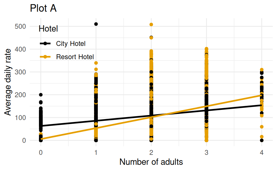
This is the original dataset:
Rows: 5
Columns: 1
$ scores <dbl> 1.563, -0.515, 1.206, -0.411, 0.523| A | B | C | D | ||||||
|---|---|---|---|---|---|---|---|---|---|
| -0.515 | 1.563 | -0.515 | -0.522 | ||||||
| -0.411 | -0.411 | -0.411 | 1.12 | ||||||
| 1.563 | -0.515 | -0.411 | 1.206 | ||||||
| -0.515 | 1.563 | 0.68 | |||||||
| -0.515 | 1.563 | 0.83 | |||||||
| 0.523 | |||||||||
| 1.563 |
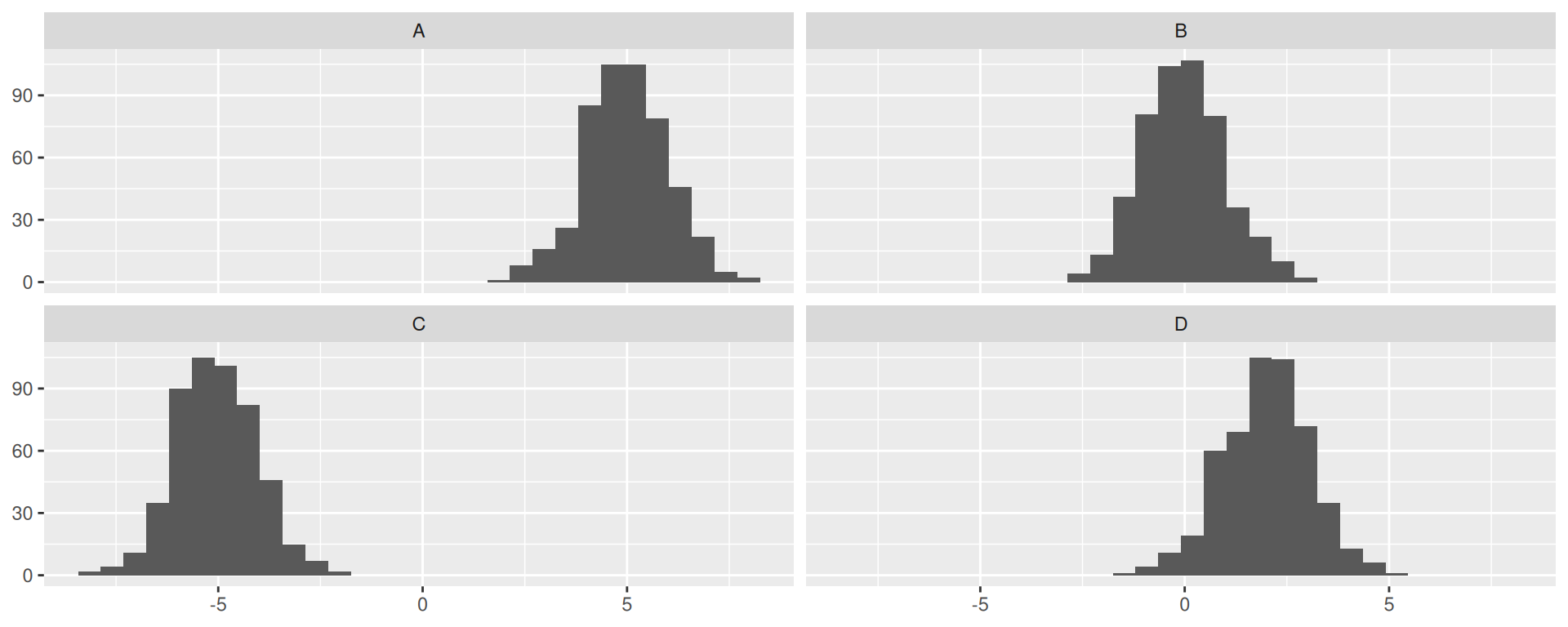
For these hypotheses
\[ \begin{aligned} H_0&: \beta_1=5\\ H_A&: \beta_1\neq 5. \end{aligned} \]
Go to your ae project in RStudio.
If you haven’t yet done so, make sure all of your changes up to this point are committed and pushed, i.e., there’s nothing left in your Git pane.
If you haven’t yet done so, click Pull to get today’s application exercise file: ae-19-card-krueger.qmd.
Work through the application exercise in class, and render, commit, and push your edits.